
 Last week at AGU, I presented the results of the project Steve Easterbrook and I worked on this summer. Click the thumbnail on the left for a full size PDF. Also, you can download the updated versions of our software diagrams:
- COSMOS (COmmunity earth System MOdelS) 1.2.1
- Model E: Oct. 11, 2011 snapshot
- HadGEM3 (Hadley Centre Global Environmental Model, version 3): August 2009 snapshot
- CESM (Community Earth System Model) 1.0.3
- GFDL (Geophysical Fluid Dynamics Laboratory), Climate Model 2.1 coupled to MOM (Modular Ocean Model) 4.1
- IPSL (Institut Pierre Simon Laplace), Climate Model 5A
- UVic ESCM (Earth System Climate Model) 2.9
And, since the most important part of poster sessions is the schpiel you give and the conversations you have, here is my schpiel:
Steve and I realized that while comparisons of the output of global climate models are very common (for example, CMIP5: Coupled Model Intercomparison Project Phase 5), nobody has really sat down and compared their software structure. We tried to fill this gap in research with a qualitative comparison study of seven models. Six of them are GCMs (General Circulation Models – the most complex climate simulations) in the CMIP5 ensemble; one, the UVic model, is not in CMIP because it’s really more of an EMIC (Earth System Model of Intermediate Complexity – simpler than a GCM). However, it’s one of the most complex EMICs, and contains a full GCM ocean, so we thought it would present an interesting boundary case. (Also, the code was easier to get access to than the corresponding GCM from Environment Canada. When we write this up into a paper we will probably use that model instead.)
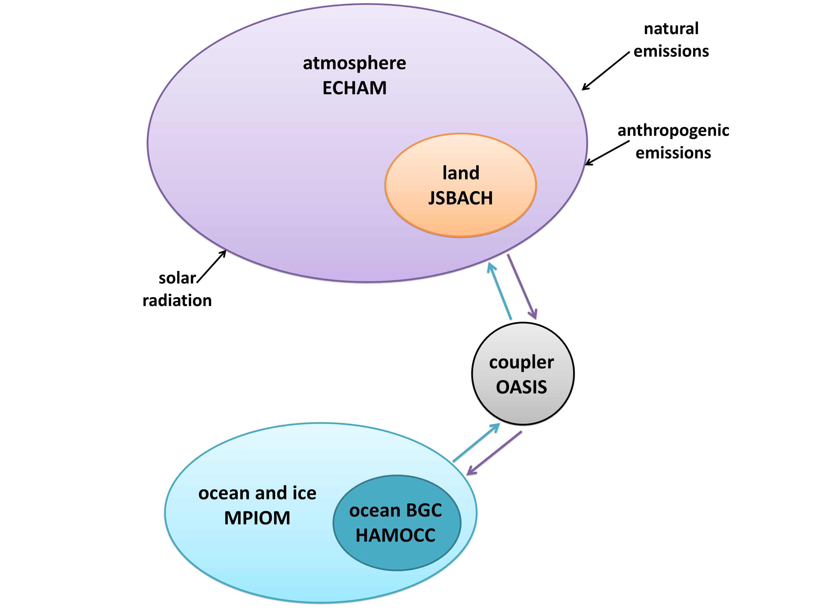
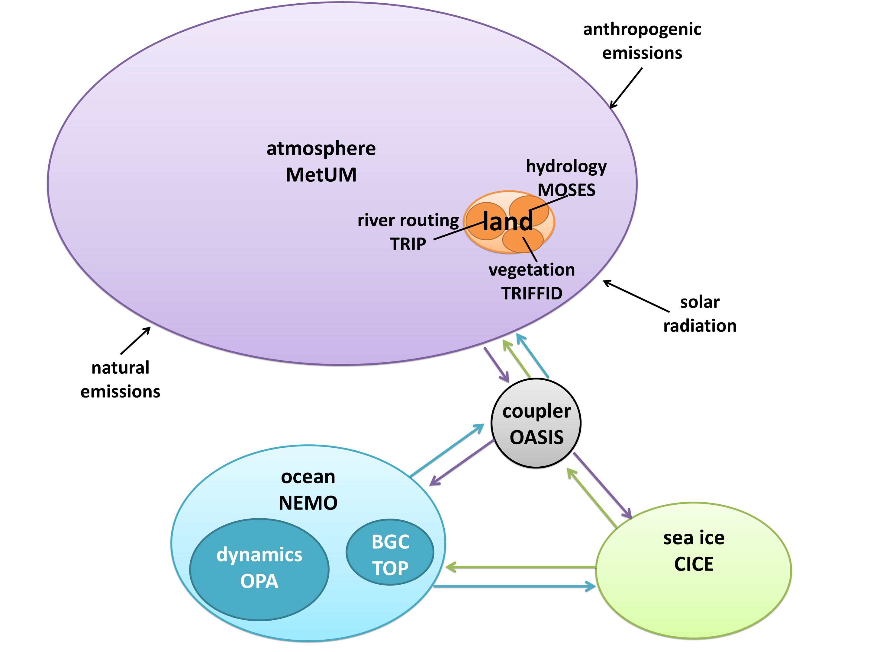
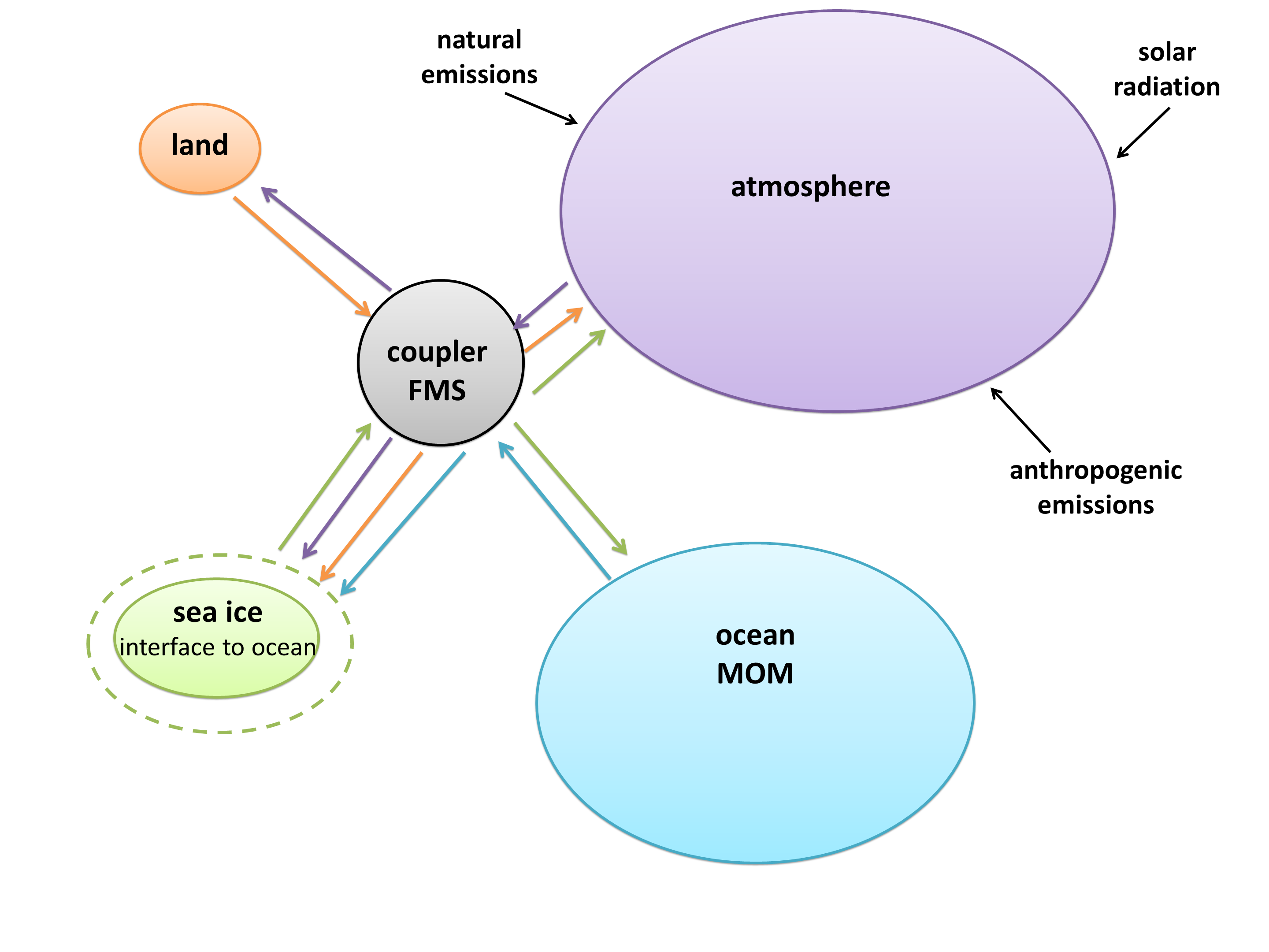
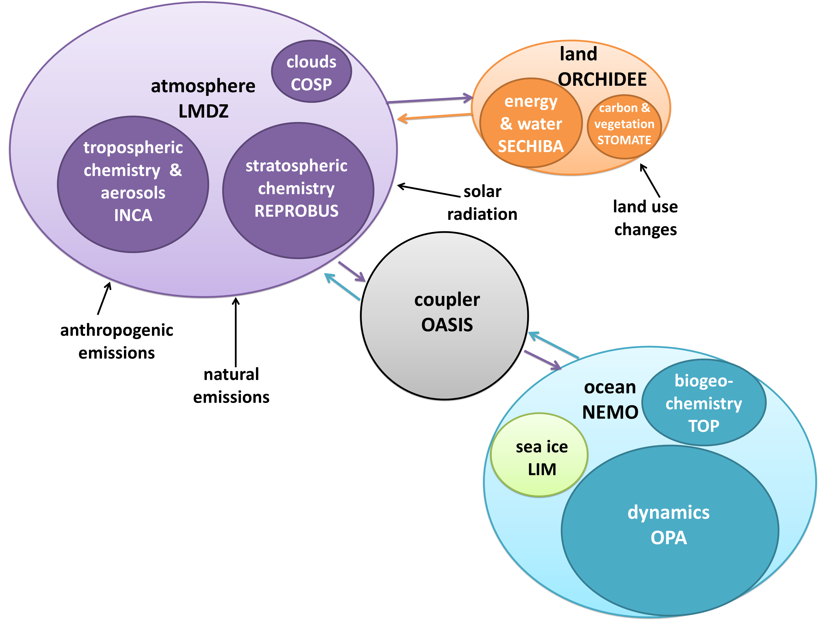
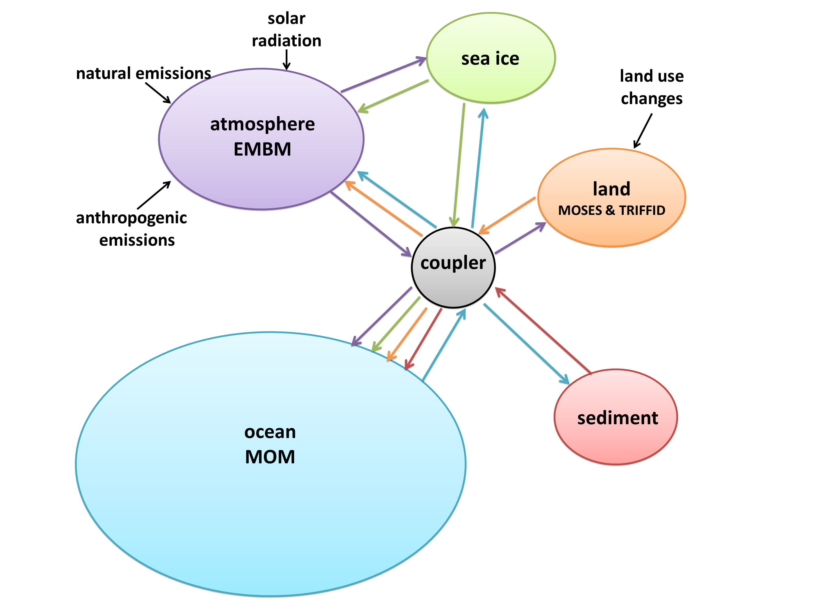
 I created a diagram of each model’s architecture. The area of each bubble is roughly proportional to the lines of code in that component, which we think is a pretty good proxy for complexity – a more complex model will have more subroutines and functions than a simple one. The bubbles are to scale within each model, but not between models, as the total lines of code in a model varies by about a factor of 10. A bit difficult to fit on a poster and still make everything readable! Fluxes from each component are represented by coloured arrows (the same colour as the bubble), and often pass through the coupler before reaching another component.
We examined the amount of encapsulation of components, which varies widely between models. CESM, on one end of the spectrum, isolates every component completely, particularly in the directory structure. Model E, on the other hand, places nearly all of its files in the same directory, and has a much higher level of integration between components. This is more difficult for a user to read, but it has benefits for data transfer.
While component encapsulation is attractive from a software engineering perspective, it poses problems because the real world is not so encapsulated. Perhaps the best example of this is sea ice. It floats on the ocean, its extent changing continuously. It breaks up into separate chunks and can form slush with the seawater. How do you split up ocean code and ice code? CESM keeps the two components completely separate, with a transient boundary between them. IPSL represents ice as an encapsulated sub-component of their ocean model, NEMO (Nucleus for European Modeling of the Ocean). COSMOS integrates both ocean and ice code together in MPI-OM (Max Planck Institute Ocean Model).
GFDL took a completely different, and rather innovative, approach. Sea ice in the GFDL model is an interface, a layer over the ocean with boolean flags in each cell indicating whether or not ice is present. All fluxes to and from the ocean must pass through the “sea ice”, even if they’re at the equator and the interface is empty.
Encapsulation requires code to tie components together, since the climate system is so interconnected. Every model has a coupler, which fulfills two main functions: controlling the main time-stepping loop, and passing data between components. Some models, such as CESM, use the coupler for every interaction. However, if two components have the same grid, no interpolation is necessary, so it’s often simpler just to pass them directly. Sometimes this means a component can be completely disconnected from the coupler, such as the land model in IPSL; other times it still uses the coupler for other interactions, such as the HadGEM3 arrangement with direct ocean-ice fluxes but coupler-controlled ocean-atmosphere and ice-atmosphere fluxes.
While it’s easy to see that some models are more complex than others, it’s also interesting to look at the distribution of complexity within a model. Often the bulk of the code is concentrated in one component, due to historical software development as well as the institution’s conscious goals. Most of the models are atmosphere-centric, since they were created in the 1970s when numerical weather prediction was the focus of the Earth system modelling community. Weather models require a very complex atmosphere but not a lot else, so atmospheric routines dominated the code. Over time, other components were added, but the atmosphere remained at the heart of the models. The most extreme example is HadGEM3, which actually uses the same atmosphere model for both weather prediction and climate simulations!
The UVic model is quite different. The University of Victoria is on the west coast of Canada, and does a lot of ocean studies, so the model began as a branch of the MOM ocean model from GFDL. The developers could have coupled it to a complex atmosphere model in an effort to mimic full GCMs, but they consciously chose not to. Atmospheric routines need very short time steps, so they eat up most of the run time, and make very long simulations not feasible. In an effort to keep their model fast, UVic created EMBM (Energy Moisture Balance Model), an extremely simple atmospheric model (for example, it doesn’t include dynamic precipitation – it simply rains as soon as a certain humidity is reached). Since the ocean is the primary moderator of climate over the long run, the UVic ESCM still outputs global long-term averages that match up nicely with GCM results.
Finally, CESM and Model E could not be described as “land-centric”, but land is definitely catching up – it’s even surpassed the ocean model in both cases! These two GCMs are cutting-edge in terms of carbon cycle feedbacks, which are primarily terrestrial, and likely very important in determining how much warming we can expect in the centuries to come. They are currently poorly understood and difficult to model, so they are a new frontier for Earth system modelling. Scientists are moving away from a binary atmosphere-ocean paradigm and towards a more comprehensive climate system representation.
I presented this work to some computer scientists in the summer, and many of them asked, “Why do you need so many models? Wouldn’t it be better to just have one really good one that everyone collaborated on?” It might be simpler from a software engineering perspective, but for the purposes of science, a variety of diverse models is actually better. It means you can pick and choose which model suits your experiment. Additionally, it increases our confidence in climate model output, because if dozens of independent models are saying the same thing, they’re more likely to be accurate than if just one model made a given prediction. Diversity in model architecture arguably produces the software engineering equivalent of perturbed physics, although it’s not systematic or deliberate.
A common question people asked me at AGU was, “Which model do you think is the best?” This question is impossible to answer, because it depends on how you define “best”, which depends on what experiment you are running. Are you looking at short-term, regional impacts at a high resolution? HadGEM3 would be a good bet. Do you want to know what the world will be like in the year 5000? Go for UVic, otherwise you will run out of supercomputer time! Are you studying feedbacks, perhaps the Paleocene-Eocene Thermal Maximum? A good choice would be CESM. So you see, every model is the best at something, and no model can be the best at everything.
You might think the ideal climate model would mimic the real world perfectly. It would still have discrete grid cells and time steps, but it would be like a digital photo, where the pixels are so small that it looks continuous even when you zoom in. It would contain every single Earth system process known to science, and would represent their connections and interactions perfectly.
Such a model would also be a nightmare to use and develop. It would run slower than real time, making predictions of the future useless. The code would not be encapsulated, so organizing teams of programmers to work on certain aspects of the model would be nearly impossible. It would use more memory than computer hardware offers us – despite the speed of computers these days, they’re still too slow for many scientific models!
We need to balance complexity with feasibility. A hierarchy of complexity is important, as is a variety of models to choose from. Perfectly reproducing the system we’re trying to model actually isn’t the ultimate goal.
Please leave your questions below, and hopefully we can start a conversation – sort of a virtual poster session!

Excellent post!
For those of us who are not completely immersed in climate modeling, please add a glossary defining all of the acronyms that are used.
Thanks for the suggestion. I put definitions inline. I have used these acronyms for so long I forget they’re not common knowledge! -Kate
This is a great post. Which journals are you considering for the paper?
We are aiming for something along the lines of Climatic Change, but if that doesn’t work out, something more specialized like Geoscientific Model Development would be our best bet. -Kate
Hi Kate,
Interesting work and nicely done.
“Wouldn’t it be better to just have one really good one that everyone collaborated on?”
I agree that a diversity of models is helpful. With that said, however, ECMWF have made huge advances by having a very talented international team work tirelessly on improving just one model. It is for that reason that ECMWF remains the best medium-range global model of all.
Perhaps this is already being done, but I would think that a similar approach would be ideal for developing a realistic climate model that can be run at high spatial and temporal resolution on a centennial time scale.
Would you be willing to post this on Skeptical Science too, Kate? If so, and if you have time, it might help to both define the acronyms and perhaps simplify the language a bit, if possible.
If you don’t have time, we could at least define the acronyms for you.
Acronyms are coming right up. A post on SkS sounds great; I will work on making a plain English version this weekend and submit it next week sometime. -Kate
Excellent, thanks Kate.
“You might think the ideal climate model would mimic the real world perfectly. It would still have discrete grid cells and time steps, but it would be like a digital photo, where the pixels are so small that it looks continuous even when you zoom in. It would contain every single Earth system process known to science, and would represent their connections and interactions perfectly.”
I’ve always said the in order to write a Really good simulation of the earth, you’d need a computer …well… the size of the earth.
Hi Kate,
Which model do you think is best for estimating global warming right through until the end of this century?
Cheers,
Martin
That’s a tough one, and certainly a subjective call. The UVic model wouldn’t be a good fit (it’s really aimed at low-resolution and long term simulations, or sensitivity studies), but any of the other six (which all did experiments like this for CMIP5) would work well. Personally, I would be tempted to go for CESM or Model E because they’re ahead of the curve on modelling terrestrial feedbacks in the carbon cycle. -Kate
Hi Kate,
Thanks for your quick reply.
Why are terrestrial feedbacks in the carbon cycle so important? I mean I know that burning fossil fuels adds CO2 to the atmosphere. And I know that a lot of the CO2 is then adsorbed by the oceans. So why is land important?
Cheers,
Martin
There are certain terrestrial carbon cycle feedbacks that were likely very important in previous climate changes (such as the PETM) but which are poorly understood and generally not included in the models. These include the CO2 released by melting permafrost, as well as contraction of the boreal forest, one of the largest carbon sinks in the world. Positive feedbacks like this have the potential to be real game-changers for the climate.
For a long time GCMs have been a binary atmosphere-ocean structure, and land has largely been neglected, but groups like NCAR and GISS are starting to move from atmosphere-ocean circulation models to “Earth system models” which have a more comprehensive structure. -Kate
Hi Kate!
It is really interesting post! Keep up your spirit of studying our climate system.
I am Ph.D student working on climate modeling. I have been trying to study climate feedbacks for the last 18 months. Unfortunately, I didn’t get a good method to study such feedbacks. I am curious how one studies feedbacks with GCMs. I am not an ignorant but explorer for novel and best methods.
what I want to know is that inspite of a lot of research has been done so far, we are not good at understanding such processes. The existing climate models yield good results in other respect but not towards feedbacks. Could you be sure why this is happening? Any clue you got ?
Do you think and have any other novel method can be implemented to study?
There are a number of ways to study feedbacks with GCMs. One approach that has gained popularity in the last few years is the radiative kernel method. See Soden et al. (2008) for details.
Hi Kishore, sorry it took me so long to respond to your questions. Feedbacks are definitely the new frontier of climate modelling, and something I’m hoping to learn more about in the future. I think one of the reasons they are poorly understood is that observations are limited – we haven’t been able to see feedbacks in action until recent decades, and many of them (eg Arctic processes) are in difficult-to-reach areas. Unfortunately, I think by the time we understand feedbacks well, we could be in big trouble…
Keep us up to date with your research!
Kate
An interesting summary of a lot of complex information. I have a question and a suggestion. I’m interested in what software you used to create the poster.
I’d also like to suggest that you include how each of the systems models the Earth. Spherical? Oblate? and how they partition the surface for analysis. Rectangles?Squares?Triangles?
The software diagrams themselves were created on Microsoft PowerPoint. In retrospect I think something like Illustrator would be better, but Adobe products seem to hate my computer…that’s a long story for another time.
An earlier version of the poster (for a university function) was created in PowerPoint as well, and I tried to alter it to fit the AGU size requirements, but unfortunately PowerPoint has a size restriction. Making a smaller poster, then saving it as a larger PDF, didn’t work…another long story. In the end, I went with Libre Office Impress, the PowerPoint alternative that comes with Ubuntu. It’s not as “pretty” as MS Office products, but it cooperated with me. Next time I will just start with that!
Comparing grids was beyond the scope of this study, but it’s a good idea for future work. Thanks for the suggestion.
Congratulations on a nice poster Kaitlin. I’m planning to show your bubble diagrams to my climate modeling class at University of Washington in a few weeks. Good luck with your studies.
Hi Kate,
I just found this page and printed the page cause this page is useful for me.
Currently, I’m studying climate change impacts to agriculture yields…so I need estimated some climate variables under scenarios.
a. The first step is to find future climate variables using either GCM or RegCM,
b. the results of future climate models…will be inputted into a crop model to get crop yields due to climate change.
Could you suggest which the model I shall use to estimate climate variables ?
Any suggestion to my steps /
Bahri,
A PhD student
Victoria Business School
Victoria Univ of Wellington
New Zealand
What is it about climate models, which have so much in common structurally and functionally with weather models, that allows them to predict climate so convincingly for decades in advance when the best that weather models can do is predict weather some ten days in advance? I should think that the weathermen would be falling all over themselves to get hold of the climate scientists’ code in the interest of being able to make longer-term forecasts! Or am I missing something?