
I haven’t forgotten about this project! Read the introduction and ODE derivation if you haven’t already.
Last time I derived the following ODE for temperature T at time t:
where S and τ are constants, and F(t) is the net radiative forcing at time t. Eventually I will discuss each of these terms in detail; this post will focus on S.
At equilibrium, when dT/dt = 0, the ODE necessitates T(t) = S F(t). A physical interpretation for S becomes apparent: it measures the equilibrium change in temperature per unit forcing, also known as climate sensitivity.
A great deal of research has been conducted with the aim of quantifying climate sensitivity, through paleoclimate analyses, modelling experiments, and instrumental data. Overall, these assessments show that climate sensitivity is on the order of 3 K per doubling of CO2 (divide by 5.35 ln 2 W/m2 to convert to warming per unit forcing).
The IPCC AR4 report (note that AR5 was not yet published at the time of my calculations) compared many different probability distribution functions (PDFs) of climate sensitivity, shown below. They follow the same general shape of a shifted distribution with a long tail to the right, and average 5-95% confidence intervals of around 1.5 to 7 K per doubling of CO2.

Box 10.2, Figure 1 of the IPCC AR4 WG1: Probability distribution functions of climate sensitivity (a), 5-95% confidence intervals (b).
These PDFs generally consist of discrete data points that are not publicly available. Consequently, sampling from any existing PDF would be difficult. Instead, I chose to create my own PDF of climate sensitivity, modelled as a log-normal distribution (e raised to the power of a normal distribution) with the same shape and bounds as the existing datasets.
The challenge was to find values for μ and σ, the mean and standard deviation of the corresponding normal distribution, such that for any z sampled from the log-normal distribution,


Since erf, the error function, cannot be evaluated analytically, this two-parameter problem must be solved numerically. I built a simple particle swarm optimizer to find the solution, which consistently yielded results of μ = 1.1757, σ = 0.4683.
The upper tail of a log-normal distribution is unbounded, so I truncated the distribution at 10 K, consistent with existing PDFs (see figure above). At the beginning of each simulation, climate sensitivity in my model is sampled from this distribution and held fixed for the entire run. A histogram of 106 sampled points, shown below, has the desired characteristics.
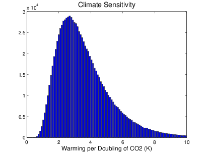
Histogram of 106 points sampled from the log-normal distribution used for climate sensitivity in the model.
Note that in order to be used in the ODE, the sampled points must then be converted to units of Km2/W (warming per unit forcing) by dividing by 5.35 ln 2 W/m2, the forcing from doubled CO2.

If the estimate of climate sensitivity is 3K per doubling of carbon dioxide, how is that moderated to reflect non greenhouse gas factors that do not apply linearly – for example – ice albedo feedback? Isn’t it necessary to consider such factors?
I also think sometimes the climate sensitivity can be misleading (and certainly taken out of context when people claim it’s too low) as I presume it really just makes a statement about adding x amount of carbon dioxide without accounting for feedbacks that may add more. For example, much of the IPCC extrapolation is based on human emission projections without necessarily adequately considering carbon from various reservoirs such as melting permafrost, decaying clathrates, changing landscapes (forest die off/burning), etc.
To that extent it doesn’t give a good guide for “if we release x ppm carbon dioxide then we should expect y warming” – as much of these feedbacks are dependent upon circumstances. In short I’m not sure how helpful a concept climate sensitivity is as a single value?
The climate sensitivity described above does account for climate feedbacks, particularly water vapor / lapse rate, clouds, and snow/ice albedo. Without feedbacks, it would be about 1 K.
But this does not typically include carbon cycle feedbacks like permafrost and clathrates, and may not correctly extrapolate some feedbacks (like land surface albedo changes from ecosystem dynamics). And, as you say, it is somewhat state- and path-dependent (but perhaps not dramatically so).
So yes, climate sensitivity isn’t the whole story. But it’s probably a good first-order approximation to the surface temperature response over the next century, barring major surprises. (Also, I think Kaitlin is planning to introduce a simple carbon cycle feedback into her model.)
Great post.
Dr.A.Jagadeesh Nellore(AP),india
You state: At equilibrium, when dT/dt = 0, the ODE necessitates T(t) = S F(t).
An alternative view obtained from integrating your ODE is that
T(t) = S F / tau – S dF/dt + …
When F is constant the dF/dt and higher derivatives are zero so necessarily T tends to
T(t) = S F
You may find that looking at an analytical solution to the ODE (via an integrating factor) will give you physical insight into the output of your model and help with verification (ie is it producing the expected output). Interesting integrable forms for F which approximate real cases are F = a, F = a t, F = a t^2, F = sin(a t), F = exp(a t).
I’m not sure I agree with the PDF you presented – it places the same probability that doubling causes ~4.0°C warming as about 1.8°C… I don’t think that this jives with most recent estimates of climate sensitivity but more so the tail is too long – the probability that a doubling in CO2 causes 6 degrees warming is way too high.