
During our time in Australia, my partner and I decided on a whim to spend a weekend in the Blue Mountains. This national park, a two-hour train ride west of Sydney, forms part of the Great Dividing Range: a chain of mountains which stretches from north to south across the entire country, separating the vast outback to the west from the narrow strip of coastal rainforest to the east.
For a region so close to Sydney, the Blue Mountains feel surprisingly remote. You can stand at any number of clifftops, gaze out over a seemingly endless stretch of land, and see no sign of civilization whatsoever. Or you can walk down into the valleys between the mountains and explore the rainforest, a vast expanse of ancient gumtrees that’s managed to hide koalas previously thought to have vanished, and possibly even an escaped panther.
 Four months later, when we were safely back in Canada, the Blue Mountains bushfires began. It was October, barely even spring in the Southern Hemisphere. To have fires starting so early in the season was virtually unheard of.
The triggers for the fires were decidedly human-caused: arson, a botched army exercise, and sparking power lines. However, unusually hot, dry, and windy conditions allowed the fires to spread far more quickly than they would have in a more normal October.
To get from the clifftops of Echo Point to the walking trails in the valley below, we took the Giant Stairway, which is exactly what it sounds like. Imagine the steepest and narrowest stairway you can manage, cut into the stone cliff and reinforced with metal, and a handrail which you cling to for dear life. Make it 902 stairs long (by my count, so let’s say plus or minus 5) and wind it back and forth around the cliff. After a few minutes walking down the stairway your knees start to buckle, and you require more and longer breaks, but you still can’t see the bottom.
The exhaustion is worth it simply due to the view.

Sometimes we would see swarms of sulfur-crested cockatoos flying over the treetops hundreds of metres below. They looked like tiny white specks at such a distance, but we could still hear them squawking to one another.
The bushfires of 2013 didn’t affect any of the areas we visited in the Blue Mountains – in fact, none of the main tourism regions were damaged. The main losses occurred in residential areas in and around the Blue Mountains. As of October 19th, 208 houses and 40 non-residential buildings had been destroyed.
Despite the huge amount of property loss, there were only two fatalities from the bushfires. This relatively successful outcome was due to mass evacuations organized by the government of New South Wales. At one point a state of emergency was declared, which authorized police to force residents to leave their houses.
As the fires continued to burn out of control, westerly winds blew the smoke and ash right over Sydney. During sunsets the sky over Sydney Harbour turned a bright orange, giving the illusion of a city built on the surface of Mars.

 I had heard about lyre birds, widely considered to be among the best mimics of the animal kingdom, many times before. In an elaborate courtship display, the male lyre bird perfectly imitates the songs of nearly every other bird in the forest, one after another like some kind of avian pop-music mashup. Lyre birds blow mockingbirds right out of the water.
Footage from the BBC of a lyre bird imitating camera shutters and chainsaws seemed too good to be true, but its authenticity was bolstered by a similar story from my friend at the climate lab in Sydney. Her neighbours had been doing renovations, and when they were finished the construction equipment went away but the sounds kept going. That’s when they discovered the lyre bird living in the garden.
We saw three or four lyre birds while hiking in the valley that weekend, but for the most part they just wandered around the forest floor, combing through the leaf litter with an outstretched foot and keeping their beaks firmly shut. It was winter in Australia, after all – not courtship season for most birds. On the last day of hiking, we sat by the side of the trail for a rest and a drink of water, while my partner quizzed me on the local bird calls.
“What kind of bird is making that song?”
“An eastern whip-bird, I think.
“Hang on, it just changed into a kookaburra.
“And now it’s a currawong?”
A few minutes later, a male lyre bird strolled out onto the path ahead of us, showing off his fantastic tail feathers and looking extremely pleased with himself.
It is well known among scientists that human-caused climate change increases the risk of severe bushfires. Spells of hot weather will obviously become more common as the planet warms, but so will prolonged droughts, especially in subtropical regions like Australia. Add an initial trigger, like a lightning strike or an abandoned campfire, and you have the perfect recipe for a bushfire.
The current Australian government, which has a history of questionable statements on climate change, really doesn’t want to believe this. Prime Minister Tony Abbott asserted that “these fires are certainly not a function of climate change, they’re a function of life in Australia”, while Environment Minister Greg Hunt cited Wikipedia during a similar statement. I was actually heartened by these events: the ensuing public outcry convinced me that Australians, by and large, do not buy into their government’s indifference on this issue.
It came as a surprise to nobody in the climate science community, and probably nobody in Australia, that 2013 was Australia’s warmest year on record. The previous record, set in 2005, was exceeded by a fairly significant 0.17°C. Even more remarkable was the fact that 2013 was an ENSO-neutral year. For Australia to shatter this temperature record without the help of El Niño indicates that something else (*cough cough climate change*) is at work.
Would the Blue Mountains bushfires have been so devastating without the help of human-caused climate change? In a cooler and wetter October, closer to the historical average, would the initial fire triggers have developed into anything significant? We’ll never know for sure. What we can say, though, is that bushfires like these will only become more common as climate change continues. This is what the future will look like.


 = E")


- O(t)")
 - \epsilon \sigma T_1(t)^4")
)}{dt} = I(t) - \epsilon \sigma (T_0 + T(t))^4")
 - \epsilon \sigma T_0^4 (1 + \tfrac{T(t)}{T_0})^4")
![c \: \frac{dT}{dt} = I(t) - \epsilon \sigma T_0^4 (1 + 4 \tfrac{T(t)}{T_0} + O[(\tfrac{T(t)}{T_0})^2])](https://s0.wp.com/latex.php?latex=c+%5C%3A+%5Cfrac%7BdT%7D%7Bdt%7D+%3D+I%28t%29+-+%5Cepsilon+%5Csigma+T_0%5E4+%281+%2B+4+%5Ctfrac%7BT%28t%29%7D%7BT_0%7D+%2B+O%5B%28%5Ctfrac%7BT%28t%29%7D%7BT_0%7D%29%5E2%5D%29+&bg=ffffff&fg=333333&s=1 "c \: \frac{dT}{dt} = I(t) - \epsilon \sigma T_0^4 (1 + 4 \tfrac{T(t)}{T_0} + O[(\tfrac{T(t)}{T_0})^2])")
 - \epsilon \sigma T_0^4 (1 + 4 \tfrac{T(t)}{T_0})")
 - \epsilon \sigma T_0^4 - 4 \epsilon \sigma T_0^3 T(t)")
 - O_0 - 4 \epsilon \sigma T_0^3 T(t)")
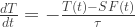
 - 4 \epsilon \sigma T_0^3 T(t)}{c}")
 - \tfrac{1}{4 \epsilon \sigma T_0^3} F(t)}{\tfrac{c}{4 \epsilon \sigma T_0^3}}")

