Climate change and the jet stream

Here in the northern mid-latitudes (much of Canada and the US, Europe, and the northern half of Asia) our weather is governed by the jet stream. This high-altitude wind current, flowing rapidly from west to east, separates cold Arctic air (to the north) from warmer temperate air (to the south). So on a given day, if you’re north of the jet stream, the weather will probably be cold; if you’re to the south, it will probably be warm; and if the jet stream is passing over you, you’re likely to get rain or snow.

The jet stream isn’t straight, though; it’s rather wavy in the north-south direction, with peaks and troughs. So it’s entirely possible for Calgary to experience a cold spell (sitting in a trough of the jet stream) while Winnipeg, almost directly to the east, has a heat wave (sitting in a peak). The farther north and south these peaks and troughs extend, the more extreme these temperature anomalies tend to be.

Sometimes a large peak or trough will hang around for weeks on end, held in place by certain air pressure patterns. This phenomenon is known as “blocking”, and is often associated with extreme weather. For example, the 2010 heat wave in Russia coincided with a large, stationary, long-lived peak in the polar jet stream. Wildfires, heat stroke, and crop failure ensued. Not a pretty picture.

As climate change adds more energy to the atmosphere, it would be naive to expect all the wind currents to stay exactly the same. Predicting the changes is a complicated business, but a recent study by Jennifer Francis and Stephen Vavrus made headway on the polar jet stream. Using North American and North Atlantic atmospheric reanalyses (models forced with observations rather than a spin-up) from 1979-2010, they found that Arctic amplification – the faster rate at which the Arctic warms, compared to the rest of the world – makes the jet stream slower and wavier. As a result, blocking events become more likely.

Arctic amplification occurs because of the ice-albedo effect: there is more snow and ice available in the Arctic to melt and decrease the albedo of the region. (Faster-than-average warming is not seen in much of Antarctica, because a great deal of thermal inertia is provided to the continent in the form of strong circumpolar wind and ocean currents.) This amplification is particularly strong in autumn and winter.

Now, remembering that atmospheric pressure is directly related to temperature, and pressure decreases with height, warming a region will increase the height at which pressure falls to 500 hPa. (That is, it will raise the 500 hPa “ceiling”.) Below that, the 1000 hPa ceiling doesn’t rise very much, because surface pressure doesn’t usually go much above 1000 hPa anyway. So in total, the vertical portion of the atmosphere that falls between 1000 and 500 hPa becomes thicker as a result of warming.

Since the Arctic is warming faster than the midlatitudes to the south, the temperature difference between these two regions is smaller. Therefore, the difference in 1000-500 hPa thickness is also smaller. Running through a lot of complicated physics equations, this has two main effects:

  1. Winds in the east-west direction (including the jet stream) travel more slowly.
  2. Peaks of the jet stream are pulled farther north, making the current wavier.

Also, both of these effects reinforce each other: slow jet streams tend to be wavier, and wavy jet streams tend to travel more slowly. The correlation between relative 1000-500 hPa thickness and these two effects is not statistically significant in spring, but it is in the other three seasons. Also, melting sea ice and declining snow cover on land are well correlated to relative 1000-500 hPa thickness, which makes sense because these changes are the drivers of Arctic amplification.

Consequently, there is now data to back up the hypothesis that climate change is causing more extreme fall and winter weather in the mid-latitudes, and in both directions: unusual cold as well as unusual heat. Saying that global warming can cause regional cold spells is not a nefarious move by climate scientists in an attempt to make every possible outcome support their theory, as some paranoid pundits have claimed. Rather, it is another step in our understanding of a complex, non-linear system with high regional variability.

Many recent events, such as record snowfalls in the US during the winters of 2009-10 and 2010-11, are consistent with this mechanism – it’s easy to see that they were caused by blocking in the jet stream when Arctic amplification was particularly high. They may or may not have happened anyway, if climate change wasn’t in the picture. However, if this hypothesis endures, we can expect more extreme weather from all sides – hotter, colder, wetter, drier – as climate change continues. Don’t throw away your snow shovels just yet.

Advertisement

How do climate models work?

Also published at Skeptical Science

This is a climate model:

T = [(1-α)S/(4εσ)]1/4

(T is temperature, α is the albedo, S is the incoming solar radiation, ε is the emissivity, and σ is the Stefan-Boltzmann constant)

An extremely simplified climate model, that is. It’s one line long, and is at the heart of every computer model of global warming. Using basic thermodynamics, it calculates the temperature of the Earth based on incoming sunlight and the reflectivity of the surface. The model is zero-dimensional, treating the Earth as a point mass at a fixed time. It doesn’t consider the greenhouse effect, ocean currents, nutrient cycles, volcanoes, or pollution.

If you fix these deficiencies, the model becomes more and more complex. You have to derive many variables from physical laws, and use empirical data to approximate certain values. You have to repeat the calculations over and over for different parts of the Earth. Eventually the model is too complex to solve using pencil, paper and a pocket calculator. It’s necessary to program the equations into a computer, and that’s what climate scientists have been doing ever since computers were invented.

A pixellated Earth

Today’s most sophisticated climate models are called GCMs, which stands for General Circulation Model or Global Climate Model, depending on who you talk to. On average, they are about 500 000 lines of computer code long, and mainly written in Fortran, a scientific programming language. Despite the huge jump in complexity, GCMs have much in common with the one-line climate model above: they’re just a lot of basic physics equations put together.

Computers are great for doing a lot of calculations very quickly, but they have a disadvantage: computers are discrete, while the real world is continuous. To understand the term “discrete”, think about a digital photo. It’s composed of a finite number of pixels, which you can see if you zoom in far enough. The existence of these indivisible pixels, with clear boundaries between them, makes digital photos discrete. But the real world doesn’t work this way. If you look at the subject of your photo with your own eyes, it’s not pixellated, no matter how close you get – even if you look at it through a microscope. The real world is continuous (unless you’re working at the quantum level!)

Similarly, the surface of the world isn’t actually split up into three-dimensional cells (you can think of them as cubes, even though they’re usually wedge-shaped) where every climate variable – temperature, pressure, precipitation, clouds – is exactly the same everywhere in that cell. Unfortunately, that’s how scientists have to represent the world in climate models, because that’s the only way computers work. The same strategy is used for the fourth dimension, time, with discrete “timesteps” in the model, indicating how often calculations are repeated.

It would be fine if the cells could be really tiny – like a high-resolution digital photo that looks continuous even though it’s discrete – but doing calculations on cells that small would take so much computer power that the model would run slower than real time. As it is, the cubes are on the order of 100 km wide in most GCMs, and timesteps are on the order of hours to minutes, depending on the calculation. That might seem huge, but it’s about as good as you can get on today’s supercomputers. Remember that doubling the resolution of the model won’t just double the running time – instead, the running time will increase by a factor of sixteen (one doubling for each dimension).

Despite the seemingly enormous computer power available to us today, GCMs have always been limited by it. In fact, early computers were developed, in large part, to facilitate atmospheric models for weather and climate prediction.

Cracking the code

A climate model is actually a collection of models – typically an atmosphere model, an ocean model, a land model, and a sea ice model. Some GCMs split up the sub-models (let’s call them components) a bit differently, but that’s the most common arrangement.

Each component represents a staggering amount of complex, specialized processes. Here are just a few examples from the Community Earth System Model, developed at the National Center for Atmospheric Research in Boulder, Colorado:

  • Atmosphere: sea salt suspended in the air, three-dimensional wind velocity, the wavelengths of incoming sunlight
  • Ocean: phytoplankton, the iron cycle, the movement of tides
  • Land: soil hydrology, forest fires, air conditioning in cities
  • Sea Ice: pollution trapped within the ice, melt ponds, the age of different parts of the ice

Each component is developed independently, and as a result, they are highly encapsulated (bundled separately in the source code). However, the real world is not encapsulated – the land and ocean and air are very interconnected. Some central code is necessary to tie everything together. This piece of code is called the coupler, and it has two main purposes:

  1. Pass data between the components. This can get complicated if the components don’t all use the same grid (system of splitting the Earth up into cells).
  2. Control the main loop, or “time stepping loop”, which tells the components to perform their calculations in a certain order, once per time step.

For example, take a look at the IPSL (Institut Pierre Simon Laplace) climate model architecture. In the diagram below, each bubble represents an encapsulated piece of code, and the number of lines in this code is roughly proportional to the bubble’s area. Arrows represent data transfer, and the colour of each arrow shows where the data originated:
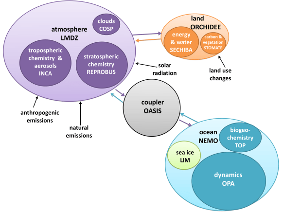
We can see that IPSL’s major components are atmosphere, land, and ocean (which also contains sea ice). The atmosphere is the most complex model, and land is the least. While both the atmosphere and the ocean use the coupler for data transfer, the land model does not – it’s simpler just to connect it directly to the atmosphere, since it uses the same grid, and doesn’t have to share much data with any other component. Land-ocean interactions are limited to surface runoff and coastal erosion, which are passed through the atmosphere in this model.

You can see diagrams like this for seven different GCMs, as well as a comparison of their different approaches to software architecture, in this summary of my research.

Show time

When it’s time to run the model, you might expect that scientists initialize the components with data collected from the real world. Actually, it’s more convenient to “spin up” the model: start with a dark, stationary Earth, turn the Sun on, start the Earth spinning, and wait until the atmosphere and ocean settle down into equilibrium. The resulting data fits perfectly into the cells, and matches up really nicely with observations. It fits within the bounds of the real climate, and could easily pass for real weather.

Scientists feed input files into the model, which contain the values of certain parameters, particularly agents that can cause climate change. These include the concentration of greenhouse gases, the intensity of sunlight, the amount of deforestation, and volcanoes that should erupt during the simulation. It’s also possible to give the model a different map to change the arrangement of continents. Through these input files, it’s possible to recreate the climate from just about any period of the Earth’s lifespan: the Jurassic Period, the last Ice Age, the present day…and even what the future might look like, depending on what we do (or don’t do) about global warming.

The highest resolution GCMs, on the fastest supercomputers, can simulate about 1 year for every day of real time. If you’re willing to sacrifice some complexity and go down to a lower resolution, you can speed things up considerably, and simulate millennia of climate change in a reasonable amount of time. For this reason, it’s useful to have a hierarchy of climate models with varying degrees of complexity.

As the model runs, every cell outputs the values of different variables (such as atmospheric pressure, ocean salinity, or forest cover) into a file, once per time step. The model can average these variables based on space and time, and calculate changes in the data. When the model is finished running, visualization software converts the rows and columns of numbers into more digestible maps and graphs. For example, this model output shows temperature change over the next century, depending on how many greenhouse gases we emit:

Predicting the past

So how do we know the models are working? Should we trust the predictions they make for the future? It’s not reasonable to wait for a hundred years to see if the predictions come true, so scientists have come up with a different test: tell the models to predict the past. For example, give the model the observed conditions of the year 1900, run it forward to 2000, and see if the climate it recreates matches up with observations from the real world.

This 20th-century run is one of many standard tests to verify that a GCM can accurately mimic the real world. It’s also common to recreate the last ice age, and compare the output to data from ice cores. While GCMs can travel even further back in time – for example, to recreate the climate that dinosaurs experienced – proxy data is so sparse and uncertain that you can’t really test these simulations. In fact, much of the scientific knowledge about pre-Ice Age climates actually comes from models!

Climate models aren’t perfect, but they are doing remarkably well. They pass the tests of predicting the past, and go even further. For example, scientists don’t know what causes El Niño, a phenomenon in the Pacific Ocean that affects weather worldwide. There are some hypotheses on what oceanic conditions can lead to an El Niño event, but nobody knows what the actual trigger is. Consequently, there’s no way to program El Niños into a GCM. But they show up anyway – the models spontaneously generate their own El Niños, somehow using the basic principles of fluid dynamics to simulate a phenomenon that remains fundamentally mysterious to us.

In some areas, the models are having trouble. Certain wind currents are notoriously difficult to simulate, and calculating regional climates requires an unaffordably high resolution. Phenomena that scientists can’t yet quantify, like the processes by which glaciers melt, or the self-reinforcing cycles of thawing permafrost, are also poorly represented. However, not knowing everything about the climate doesn’t mean scientists know nothing. Incomplete knowledge does not imply nonexistent knowledge – you don’t need to understand calculus to be able to say with confidence that 9 x 3 = 27.

Also, history has shown us that when climate models make mistakes, they tend to be too stable, and underestimate the potential for abrupt changes. Take the Arctic sea ice: just a few years ago, GCMs were predicting it would completely melt around 2100. Now, the estimate has been revised to 2030, as the ice melts faster than anyone anticipated:

Answering the big questions

At the end of the day, GCMs are the best prediction tools we have. If they all agree on an outcome, it would be silly to bet against them. However, the big questions, like “Is human activity warming the planet?”, don’t even require a model. The only things you need to answer those questions are a few fundamental physics and chemistry equations that we’ve known for over a century.

You could take climate models right out of the picture, and the answer wouldn’t change. Scientists would still be telling us that the Earth is warming, humans are causing it, and the consequences will likely be severe – unless we take action to stop it.

The Pitfalls of General Reporting: A Case Study

Today’s edition of Nature included an alarming paper, indicating record ozone loss in the Arctic due to an unusually long period of cold temperatures in the lower stratosphere.

On the same day, coverage of the story by the Canadian Press included a fundamental error that is already contributing to public confusion about the reality of climate change.

Counter-intuitively, while global warming causes temperatures in the troposphere (the lowest layer of the atmosphere) to rise, it causes temperatures in the stratosphere (the next layer up), as well as every layer above that, to fall. The exact mechanics are complex, but the pattern of a warming troposphere and a cooling stratosphere has been both predicted and observed.

This pattern was observed in the Arctic this year. As the Nature paper mentions, the stratosphere was unusually cold in early 2011. The surface temperatures, however, were unusually warm, as data from NASA shows:

Mar-May 2011

Dec-Feb 2011

While we can’t know for sure whether or not the unusual stratospheric conditions were caused by climate change, this chain of cause and effect is entirely consistent with what we can expect in a warming world.

However, if all you read was an article by the Canadian Press, you could be forgiven for thinking differently.

The article states that the ozone loss was “caused by an unusually prolonged period of extremely low temperatures.” I’m going to assume that means surface temperatures, because nothing else is specified – and virtually every member of the public would assume that too. As we saw from the NASA maps, though, cold surface temperatures couldn’t be further from the truth.

The headline, which was probably written by the Winnipeg Free Press, rather than the Canadian Press, tops off the glaring misconception nicely:

Record Ozone loss over the Arctic caused by extremely cold weather: scientists

No, no, no. Weather happens in the troposphere, not the stratosphere. While the stratosphere was extremely cold, the troposphere certainly was not. It appears that the reporters assumed the word “stratosphere” in the paper’s abstract was completely unimportant. In fact, it changes the meaning of the story entirely.

The reaction to this article, as seen in the comments section, is predictable:

So with global warming our winters are colder?

First it’s global warming that is destroying Earth, now it’s being too cold?! I’m starting to think these guys know as much about this as weather guys know about forecasting the weather!

Al gore the biggest con man since the beginning of mankind!! This guys holdings leave a bigger carbon footprint than most small countries!!

I’m confused. I thought the north was getting warmer and that’s why the polar bears are roaming around Churchill looking for food. There isn’t ice for them to go fishing.

People are already confused, and deniers are already using this journalistic error as evidence that global warming is fake. All because a major science story was written by a general reporter who didn’t understand the study they were covering.

In Manitoba, high school students learn about the different layers of the atmosphere in the mandatory grade 10 science course. Now, reporters who can’t recall this information are writing science stories for the Canadian Press.

Beautiful Things

This is what the last few days have taught me: even if the code for climate models can seem dense and confusing, the output is absolutely amazing.

Late yesterday I discovered a page of plots and animations from the Canadian Centre for Climate Modelling and Analysis. The most recent coupled global model represented on that page is CGCM3, so I looked at those animations. I noticed something very interesting: the North Atlantic, independent of the emissions scenario, was projected to cool slightly, while the world around it warmed up. Here is an example, from the A1B scenario. Don’t worry if the animation is already at the end, it will loop:

It turns out that this slight cooling is due to the North Atlantic circulation slowing down, as is very likely to happen from large additions of freshwater that change the salinity and density of the ocean (IPCC AR4 WG1, FAQ 10.2). This freshwater could come from either increased precipitation due to climate change, or meltwater from the Arctic ending up in the North Atlantic. Of course, we hear about this all the time – the unlikely prospect of the Gulf Stream completely shutting down and Europe going into an ice age, as displayed in The Day After Tomorrow – but, until now, I hadn’t realized that even a slight slowing of the circulation could cool the North Atlantic, while Europe remained unaffected.

Then, in chapter 8 of the IPCC, I read something that surprised me: climate models generate their own El Ninos and La Ninas. Scientists don’t understand quite what triggers the circulation patterns leading to these phenomena, so how can they be in the models? It turns out that the modellers don’t have to parameterize the ENSO cycles at all: they have done such a good job of reproducing global circulation from first principles that ENSO arises by itself, even though we don’t know why. How cool is that? (Thanks to Jim Prall and Things Break for their help with this puzzle.)

Jim Prall also pointed me to an HD animation of output from the UK-Japan Climate Collaboration. I can’t seem to embed the QuickTime movie (WordPress strips out some of the necessary HTML tags) so you will have to click on the link to watch it. It’s pretty long – almost 17 minutes – as it represents an entire year of the world’s climate system, in one-hour time steps. It shows 1978-79, starting from observational data, but from there it simulates its own circulation.

I am struck by the beauty of this output – the swirling cyclonic precipitation, the steady prevailing westerlies and trade winds, the subtropical high pressure belt clear from the relative absence of cloud cover in these regions. You can see storms sprinkling across the Amazon Basin, monsoons pounding South Asia, and sea ice at both poles advancing and retreating with the seasons. Scientists didn’t explicitly tell their models to do any of this. It all appeared from first principles.

Take 17 minutes out of your day to watch it – it’s an amazing stress reliever, sort of like meditation. Or maybe that’s just me…

One more quick observation: most of you are probably familiar with the naming conventions of IPCC reports. The First Assessment Report was FAR, the second was SAR, and so on, until the acronyms started to repeat themselves, so the Fourth Assessment Report was AR4. They’ll have to follow this alternate convention until the Eighth Annual Report, which will be EAR. Maybe they’ll stick with AR8, but that would be substantially less entertaining.