It turns out that when you submit a paper to a journal like Nature Geoscience “just in case, we have nothing to lose, they’ll probably reject it straight away”…sometimes you are unexpectedly successful.
Almost four years ago I took a job as a summer student of Dr. Steve Easterbrook, in the software engineering lab of the University of Toronto. This was my first time taking part in research, but also my first time living away from home and my first time using a Unix terminal (both of which are challenging, but immensely rewarding, life skills).
These diagrams proved to be really useful communication tools: we presented our work at AGU the following December, and at NCAR about a year after that, to very positive feedback. Many climate modellers we met at these conferences were pleased to have a software diagram of the model they used (which is very useful to show during presentations), but they were generally more interested in the diagrams for other models, to see how other research groups used different software structures to solve the same problems. “I had no idea they did it like that,” was a remark I heard more than a few times.
Between my undergrad and PhD, I went back to Toronto for a month where I analysed the model code more rigorously. We made a new set of diagrams which was more accurate: the code was sorted into components based on dependency structure, and the area of each component in a given diagram was exactly proportional to the line count of its source code.
Here is the diagram we made for the GFDL-ESM2M model, which is developed at the Geophysical Fluid Dynamics Laboratory in Princeton:
We wrote this all up into a paper, submitted it to GMD, and after several months and several rounds of revision it was published just yesterday! The paper is open access, and can be downloaded for free here. It’s my first paper as lead author which is pretty exciting.
I could go on about all the interesting things we discovered while comparing the diagrams, but that’s all in the paper. Instead I wanted to talk about what’s not in the paper: the story of the long and winding journey we took to get there, from my first day as a nervous summer student in Toronto to the final publication yesterday. These are the stories you don’t read about in scientific papers, which out of necessity detail the methodology as if the authors knew exactly where they were going and got there using the shortest possible path. Science doesn’t often work like that. Science is about messing around and exploring and getting a bit lost and eventually figuring it out and feeling like a superhero when you do. And then writing it up as if it was easy.
I also wanted to express my gratitude to Steve, who has been an amazing source of support, advice, conversations, book recommendations, introductions to scientists, and career advice. I’m so happy that I got to be your student. See you before long on one continent or another!
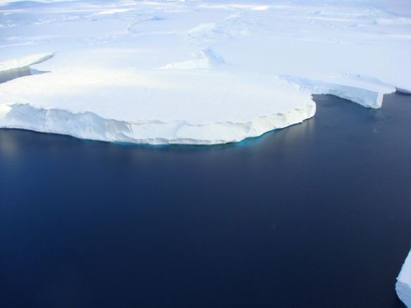
An ice sheet forms when snow falls on land, compacts into ice, and forms a system of interconnected glaciers which gradually flow downhill like play-dough. In Antarctica, it is so cold that the ice flows right into the ocean before it melts, sometimes hundreds of kilometres from the coast. These giant slabs of ice, floating on the ocean while still attached to the continent, are called ice shelves.
For an ice sheet to have constant size, the mass of ice added from snowfall must equal the mass lost due to melting and calving (when icebergs break off). Since this ice loss mainly occurs at the edges, the rate of ice loss will depend on how fast glaciers can flow towards the edges.
Ice shelves slow down this flow. They hold back the glaciers behind them in what is known as the “buttressing effect”. If the ice shelves were smaller, the glaciers would flow much faster towards the ocean, melting and calving more ice than snowfall inland could replace. This situation is called a “negative mass balance”, which leads directly to global sea level rise.
Respect the ice shelves. They are holding back disaster.
Ice shelves are perhaps the most important part of the Antarctic ice sheet for its overall stability. Unfortunately, they are also the part of the ice sheet most at risk. This is because they are the only bits touching the ocean. And the Antarctic ice sheet is not directly threatened by a warming atmosphere – it is threatened by a warming ocean.
The atmosphere would have to warm outrageously in order to melt the Antarctic ice sheet from the top down. Snowfall tends to be heaviest when temperatures are just below 0°C, but temperatures at the South Pole rarely go above -20°C, even in the summer. So atmospheric warming will likely lead to a slight increase in snowfall over Antarctica, adding to the mass of the ice sheet. Unfortunately, the ocean is warming at the same time. And a slightly warmer ocean will be very good at melting Antarctica from the bottom up.
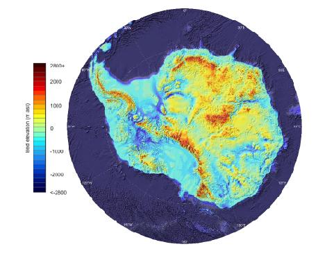
This is partly because ice melts faster in water than it does in air, even if the air and the water are the same temperature. But the ocean-induced melting will be exacerbated by some unlucky topography: over 40% of the Antarctic ice sheet (by area) rests on bedrock that is below sea level.
Elevation of the bedrock underlying Antarctica. All of the blue regions are below sea level. (Figure 9 of Fretwell et al.)
This means that ocean water can melt its way in and get right under the ice, and gravity won’t stop it. The grounding lines, where the ice sheet detaches from the bedrock and floats on the ocean as an ice shelf, will retreat. Essentially, a warming ocean will turn more of the Antarctic ice sheet into ice shelves, which the ocean will then melt from the bottom up.
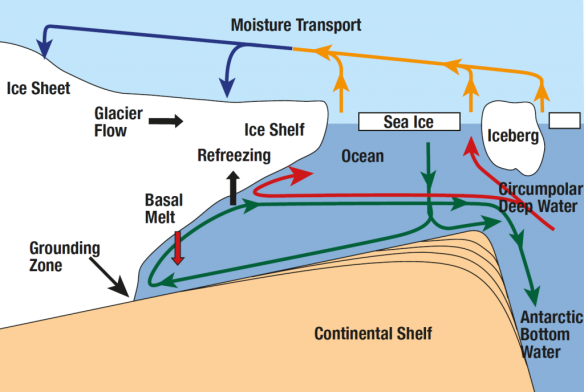
This situation is especially risky on a retrograde bed, where bedrock gets deeper below sea level as you go inland – like a giant, gently sloping bowl. Retrograde beds occur because of isostatic loading (the weight of an ice sheet pushes the crust down, making the tectonic plate sit lower in the mantle) as well as glacial erosion (the ice sheet scrapes away the surface bedrock over time). Ice sheets resting on retrograde beds are inherently unstable, because once the grounding lines reach the edge of the “bowl”, they will eventually retreat all the way to the bottom of the “bowl” even if the ocean water intruding beneath the ice doesn’t get any warmer. This instability occurs because the melting point temperature of water decreases as you go deeper in the ocean, where pressures are higher. In other words, the deeper the ice is in the ocean, the easier it is to melt it. Equivalently, the deeper a grounding line is in the ocean, the easier it is to make it retreat. In a retrograde bed, retreating grounding lines get deeper, so they retreat more easily, which makes them even deeper, and they retreat even more easily, and this goes on and on even if the ocean stops warming.
Diagram of an ice shelf on a retrograde bed (“Continental shelf”)
Which brings us to Terrifying Paper #1, by Rignot et al. A decent chunk of West Antarctica, called the Amundsen Sea Sector, is melting particularly quickly. The grounding lines of ice shelves in this region have been rapidly retreating (several kilometres per year), as this paper shows using satellite data. Unfortunately, the Amundsen Sea Sector sits on a retrograde bed, and the grounding lines have now gone past the edge of it. This retrograde bed is so huge that the amount of ice sheet it underpins would cause 1.2 metres of global sea level rise. We’re now committed to losing that ice eventually, even if the ocean stopped warming tomorrow. “Upstream of the 2011 grounding line positions,” Rignot et al., write, “we find no major bed obstacle that would prevent the glaciers from further retreat and draw down the entire basin.”
They look at each source glacier in turn, and it’s pretty bleak:
Pine Island Glacier: “A region where the bed elevation is smoothly decreasing inland, with no major hill to prevent further retreat.”
Smith/Kohler Glaciers: “Favorable to more vigorous ice shelf melt even if the ocean temperature does not change with time.”
Thwaites Glacier: “Everywhere along the grounding line, the retreat proceeds along clear pathways of retrograde bed.”
Only one small glacier, Haynes Glacier, is not necessarily doomed, since there are mountains in the way that cut off the retrograde bed.
From satellite data, you can already see the ice sheet speeding up its flow towards the coast, due to the loss of buttressing as the ice shelves thin: “Ice flow changes are detected hundreds of kilometers inland, to the flanks of the topographic divides, demonstrating that coastal perturbations are felt far inland and propagate rapidly.”
It will probably take a few centuries for the Amundsen Sector to fully disintegrate. But that 1.2 metres of global sea level rise is coming eventually, on top of what we’ve already seen from other glaciers and thermal expansion, and there’s nothing we can do to stop it (short of geoengineering). We’re going to lose a lot of coastal cities because of this glacier system alone.
Terrifying Paper #2, by Mengel & Levermann, examines the Wilkes Basin Sector of East Antarctica. This region contains enough ice to raise global sea level by 3 to 4 metres. Unlike the Amundsen Sector, we aren’t yet committed to losing this ice, but it wouldn’t be too hard to reach that point. The Wilkes Basin glaciers rest on a system of deep troughs in the bedrock. The troughs are currently full of ice, but if seawater got in there, it would melt all the way along the troughs without needing any further ocean warming – like a very bad retrograde bed situation. The entire Wilkes Basin would change from ice sheet to ice shelf, bringing along that 3-4 metres of global sea level rise.
It turns out that the only thing stopping seawater getting in the troughs is a very small bit of ice, equivalent to only 8 centimetres of global sea level rise, which Mengel & Levermann nickname the “ice plug”. As long as the ice plug is there, this sector of the ice sheet is stable; but take the ice plug away, and the whole thing will eventually fall apart even if the ocean stops warming. Simulations from an ice sheet model suggest it would take at least 200 years of increased ocean temperature to melt this ice plug, depending on how much warmer the ocean got. 200 years sounds like a long time for us to find a solution to climate change, but it actually takes much longer than that for the ocean to cool back down after it’s been warmed up.
This might sound like all bad news. And you’re right, it is. But it can always get worse. That means we can always stop it from getting worse. That’s not necessarily good news, but at least it’s empowering. The sea level rise we’re already committed to, whether it’s 1 or 2 or 5 metres, will be awful. But it’s much better than 58 metres, which is what we would get if the entire Antarctic ice sheet melted. Climate change is not an all-or-nothing situation; it falls on a spectrum. We will have to deal with some amount of climate change no matter what. The question of “how much” is for us to decide.
A problem which has plagued oceanography since the very beginning is a lack of observations. We envy atmospheric scientists with their surface stations and satellite data that monitor virtually the entire atmosphere in real time. Until very recently, all that oceanographers had to work with were measurements taken by ships. This data was very sparse in space and time, and was biased towards certain ship tracks and seasons.
A lack of observations makes life difficult for ocean modellers, because there is very little to compare the simulations to. You can’t have confidence in a model if you have no way of knowing how well it’s performing, and you can’t make many improvements to a model without an understanding of its shortcomings.
Our knowledge of the ocean took a giant leap forward in 2000, when a program called Argo began. “Argo floats” are smallish instruments floating around in the ocean that control their own buoyancy, rising and sinking between the surface and about 2000 m depth. They use a CTD sensor to measure Conductivity (from which you can easily calculate salinity), Temperature, and Depth. Every 10 days they surface and send these measurements to a satellite. Argo floats are battery-powered and last for about 4 years before losing power. After this point they are sacrificed to the ocean, because collecting them would be too expensive.
This is what an Argo float looks like while it’s being deployed:
With at least 27 countries helping with deployment, the number of active Argo floats is steadily rising. At the time of this writing, there were 3748 in operation, with good coverage everywhere except in the polar oceans:
The result of this program is a massive amount of high-quality, high-resolution data for temperature and salinity in the surface and intermediate ocean. A resource like this is invaluable for oceanographers, analogous to the global network of weather stations used by atmospheric scientists. It allows us to better understand the current state of the ocean, to monitor trends in temperature and salinity as climate change continues, and to assess the skill of ocean models.
But it’s still not good enough. There are two major shortcomings to Argo floats. First, they can’t withstand the extreme pressure in the deep ocean, so they don’t sink below about 2000 m depth. Since the average depth of the world’s oceans is around 4000 m, the Argo program is only sampling the upper half. Fortunately, a new program called Deep Argo has developed floats which can withstand pressures down to 6000 m depth, covering all but the deepest ocean trenches. Last June, two prototypes were successfully deployed off the coast of New Zealand, and the data collected so far is looking good. If all future Argo floats were of the Deep Argo variety, in five or ten years we would know as much about the deep ocean’s temperature and salinity structure as we currently know about the surface. To oceanographers, particularly those studying bottom water formation and transport, there is almost nothing more exciting than this prospect.
The other major problem with Argo floats is that they can’t handle sea ice. Even if they manage to get underneath the ice by drifting in sideways, the next time they rise to the surface they will bash into the underside of the ice, get stuck, and stay there until their battery dies. This is a major problem for scientists like me who study the Southern Ocean (surrounding Antarctica), which is largely covered with sea ice for much of the year. This ocean will be incredibly important for sea level rise, because the easiest way to destabilise the Antarctic Ice Sheet is to warm up the ocean and melt the ice shelves (the edges of the ice sheet which extend over the ocean) from below. But we can’t monitor this process using Argo data, because there is a big gap in observations over the region. There’s always the manual option – sending in scientists to take measurements – but this is very expensive, and nobody wants to go there in the winter.
Instead, oceanographers have recently teamed up with biologists to try another method of data collection, which is just really excellent:
They are turning seals into Argo floats that can navigate sea ice.
Southern elephant seals swim incredible distances in the Southern Ocean, and often dive as far as 2000 m below the surface. Scientists are utilising the seals’ natural talents to fill in the gaps in the Argo network, so far with great success. Each seal is tranquilized while a miniature CTD is glued to the fur on its head, after which it is released back into the wild. As the seal swims around, the sensors take measurements and communicate with satellites just like regular Argo floats. The next time the seal sheds its coat (once per year), the CTD falls off and the seal gets on with its life, probably wondering what that whole thing was about.
This project is relatively new and it will be a few years before it’s possible to identify trends in the data. It’s also not clear whether or not the seals tend to swim right underneath the ice shelves, where observations would be most useful. But if this dataset gains popularity among oceanographers, and seals become officially integrated into the Argo network…
I don’t really care about the panda bears. But that’s not saying this problem [climate change] isn’t serious. This is a people problem, this is a billion dead people problem. This is a national security problem. This is rewinding the clock 300 years to a time we don’t want to go back to.
– Nick Wood (spoken at a presentation I attended, and possibly slightly paraphrased as I scrambled to write it down; his profile is here)
My supervisors are so distinguished that they now exist in cartoon form! If that’s not the mark of a successful science communicator, I’m not sure what is.
It has been a very busy few months. Here are some of the things I have done since I last wrote:
Moved out of our apartment in Canada
Spent three weeks in Ireland with my partner’s family – this was great fun and featured lots of music, tide pools, castles, and sheep
Went back to Canada for six days
Mastered the art of packing checked luggage and carry-on bags so they are juuust under the weight limit
Said a lot of tearful goodbyes
Flew to Australia!
Discovered Sydney was 11°C and raining
Immediately regretted leaving all our warm sweaters behind (“It’s spring in Australia,” we said. “We won’t need these for months yet,” we said)
Saw all three animals I had missed the most – bats, lorikeets, and scientists – in the very first day
Officially enrolled as a PhD student at UNSW
Stumbled into the Sydney real estate market, where rent prices are more than double what we are used to, and only the wealthiest people can afford to buy property
Managed to find a great little apartment for rent within our budget
Bought out most of IKEA
Moved into said apartment (we’re getting good at this moving thing)
Helped to finish up 3 papers from the project Katrin, Tim, and I did last year, and 1 paper from the project Steve and I did 3 years ago
Read at least a dozen papers on interactions between Antarctic ice shelves and the Southern Ocean – my PhD project will be somewhere in this field
Gone out for climate beers (regular beers consumed by climate scientists) and discussed whether the Canadian or the Australian political system is more fundamentally broken
Swam in the ocean three times, and discovered that if you put on goggles and look underneath the water you can see FISH swimming around beneath you
Things are finally calming down now, and I should have time to write more frequently. Now that my head is not so full of flight schedules and rental agreements and shopping lists, it has a lot more space for climate science, and for topics to write about here.
I am so, so happy to be back at the CCRC. It is such a friendly, supportive, and enriching place to do research. While I miss my family and the Canadian wildlife and Canadian autumn (definitely not Canadian winter), this is the best time in my life to travel and explore the planet which I spend so much time studying, and hopefully, helping.
If you haven’t yet watched the television series Game of Thrones or read George R. R. Martin’s A Song of Ice and Fire books on which the show is based, I would urge you to get started (unless you are a small child, in which case I would urge you to wait a few years). The show and the books are both absolute masterpieces (although, as I alluded, definitely not for kids). I’m not usually a big fan of high fantasy, but the character and plot development of this series really pulled me in.
One of the most interesting parts of the series – maybe just for me – is the way the seasons work in Westeros and Essos, the continents explored in Game of Thrones. Winter and summer occur randomly, and can last anywhere from a couple of years to more than a decade. (Here a “year” is presumably defined by a complete rotation of the planet around the Sun, which can be discerned by the stars, rather than by one full cycle of the seasons.)
So what causes these random, multiyear seasons? Many people, George R. R. Martin included, brush off the causes as magical rather than scientific. To those people I say: you have no sense of fun.
After several lunchtime conversations with my friends from UNSW and U of T (few things are more fun than letting a group of climate scientists loose on a question like this), I think I’ve found a mechanism to explain the seasons. My hypothesis is simple, has been known to work on Earth, and satisfies all the criteria I can remember (I only read the books once and I didn’t take notes). I think that “winters” in Westeros are actually miniature ice ages, caused by the same orbital mechanisms which govern ice ages on Earth.
Glacial Cycles on Earth
First let’s look at how ice ages – the cold phases of glacial cycles – work on Earth. At their most basic level, glacial cycles are caused by gravity: the gravity of other planets in the solar system, which influence Earth’s orbit around the Sun. Three main orbital cycles, known as Milankovitch cycles, result:
A 100,000 year cycle in eccentricity: how elliptical (as opposed to circular) Earth’s path around the Sun is.
A 41,000 year cycle in obliquity: the degree of Earth’s axial tilt.
A 26,000 year cycle in precession: what time of year the North Pole is pointing towards the Sun.
These three cycles combine to impact the timing and severity of the seasons in each hemisphere. The way they combine is not simple: the superposition of three sinusoidal functions with different periods is generally a mess, and often one cycle will cancel out the effects of another. However, sometimes the three cycles combine to make the Northern Hemisphere winter relatively warm, and the Northern Hemisphere summer relatively cool.
These conditions are ideal for glacier growth in the Northern Hemisphere. A warmer winter, as long as it’s still below freezing, will often actually cause more snow to fall. A cool summer will prevent that snow from entirely melting. And as soon as you’ve got snow that sticks around for the entire year, a glacier can begin to form.
Then the ice-albedo feedback kicks in. Snow and ice reflect more sunlight than bare ground, meaning less solar radiation is absorbed by the surface. This makes the Earth’s average temperature go down, so even less of the glacier will melt each summer. Now the glacier is larger and can reflect even more sunlight. This positive feedback loop, or “vicious cycle”, is incredibly powerful. Combined with carbon cycle feedbacks, it caused glaciers several kilometres thick to spread over most of North America and Eurasia during the last ice age.
The conditions are reversed in the Southern Hemisphere: relatively cold winters and hot summers, which cause glaciers to recede. However, at this stage in Earth’s history, most of the continents are concentrated in the Northern Hemisphere. The south is mostly ocean, where there are no glaciers to recede. For this reason, the Northern Hemisphere is the one which controls Earth’s glacial cycles.
These ice ages don’t last forever, because sooner or later the Milankovitch cycles will combine in the opposite way: the Northern Hemisphere will have cold winters and hot summers, and its glaciers will start to recede. The ice-albedo feedback will be reversed: less snow and ice means more sunlight is absorbed, which makes the planet warmer, which means there is less snow and ice, and so on.
Glacial Cycles in Westeros?
I propose that Westeros (or rather, the unnamed planet which contains Westeros and Essos and any other undiscovered continents in Game of Thrones; let’s call it Westeros-world) experiences glacial cycles just like Earth, but the periods of the underlying Milankovitch cycles are much shorter – on the order of years to decades. This might imply the presence of very large planets close by, or a high number of planets in the solar system, or even multiple other solar systems which are close enough to exert significant gravitational attraction. As far as I know, all of these ideas are plausible, but I encourage any astronomers in the audience to chime in.
Given the climates of various regions in Game of Thrones, it’s clear that they all exist in the Northern Hemisphere: the further north you go, the colder it gets. The southernmost boundary of the known world is probably somewhere around the equator, because it never starts getting cold again as you travel south. Beyond that, the planet is unexplored, and it’s plausible that the Southern Hemisphere is mainly ocean. The concentration of continents in one hemisphere would allow Milankovitch cycles to induce glacial cycles in Westeros-world.
The glacial periods (“winter”) and interglacials (“summer”) would vary in length – again, on the scale of years to decades – and would appear random: the superposition of three different sine functions has an erratic pattern of peaks and troughs when you zoom in. Of course, the pattern of season lengths would eventually repeat itself, with a period equal to the least common multiple of the three Milankovitch cycle periods. But this least common multiple could be so large – centuries or even millennia – that the seasons would appear random on a human timescale. It’s not hard to believe that the people of Westeros, even the highly educated maesters, would fail to recognize a pattern which took hundreds or thousands of years to repeat.
Of course, within each glacial cycle there would be multiple smaller seasons as the planet revolved around the Sun – the way that regular seasons work on Earth. However, if the axial tilt of Westeros-world was sufficiently small, these regular seasons could be overwhelmed by the glacial cycles to the point where nobody would notice them.
There could be other hypotheses involving fluctuations in solar intensity, frequent volcanoes shooting sulfate aerosols into the stratosphere, or rapid carbon cycle feedbacks. But I think this one is the most plausible, because it’s known to happen on Earth (albeit on a much longer timescale). Can you find any holes? Please go nuts in the comments.
Both are about climate modelling, and both are definitely worth 10-20 minutes of your time.
The first is from Gavin Schmidt, NASA climate modeller and RealClimate author extraordinaire:
The second is from Steve Easterbrook, my current supervisor at the University of Toronto (this one is actually TEDxUofT, which is independent from TED):
After a long hiatus – much longer than I like to think about or admit to – I am finally back. I just finished the last semester of my undergraduate degree, which was by far the busiest few months I’ve ever experienced.
This was largely due to my honours thesis, on which I spent probably three times more effort than was warranted. I built a (not very good, but still interesting) model of ocean circulation and implemented it in Python. It turns out that (surprise, surprise) it’s really hard to get a numerical solution to the Navier-Stokes equations to converge. I now have an enormous amount of respect for ocean models like MOM, POP, and NEMO, which are extremely realistic as well as extremely stable. I also feel like I know the physics governing ocean circulation inside out, which will definitely be useful going forward.
Convocation is not until early June, so I am spending the month of May back in Toronto working with Steve Easterbrook. We are finally finishing up our project on the software architecture of climate models, and writing it up into a paper which we hope to submit early this summer. It’s great to be back in Toronto, and to have a chance to revisit all of the interesting places I found the first time around.
In August I will be returning to Australia to begin a PhD in Climate Science at the University of New South Wales, with Katrin Meissner and Matthew England as my supervisors. I am so, so excited about this. It was a big decision to make but ultimately I’m confident it was the right one, and I can’t wait to see what adventures Australia will bring.