A Visit to NCAR

Last week I was lucky enough to attend the Second Workshop on Coupling Technologies for Earth System Models, held at the National Center for Atmospheric Research (NCAR) in Boulder, Colorado, USA. I was excited just to visit NCAR, which is one of the top climate research facilities in the world. Not only is it packed full of interesting scientists and great museum displays, but it’s nestled in the Rocky Mountains and so the view from the conference room looks like this:

2013-02-21 13.46.43

Many of the visitors would spend large portions of the coffee breaks just staring out the window…

The conference was focused on couplers – the part of a climate model that ties all the other components (atmosphere, ocean, land, etc.) together. However, the presentations covered (as Rob Jacob put it) “everything that physical scientists don’t care about unless it stops working”. Since I consider myself a physical scientist, this included a lot of concepts I hadn’t thought about before:

  • Parallel processing: Since climate models are so big, it makes sense to multitask by splitting the work over many computer processors. You have to allocate the right number of processors to each component, though: if the atmosphere has too many processors, it will finish its timestep too quickly and sit there waiting until the ocean is done, and vice versa. This is called load balancing, and it gets very tricky as soon as the number of components exceeds two.
  • Scalability: The more processors you use, the faster the model runs, but the speed has diminishing returns. If you double the number of processors, you won’t quite double the speed, particularly if the number of processors exceeds 104 (a setup which is becoming increasingly affordable for large research groups). Historically, the coupler has not been a code bottleneck (limiting factor for model speed), but as the number of processors gets very large, that scenario is changing. We have to figure out the most efficient way to couple many small components together, so that climate model speed can continue to keep up with advances in computer hardware.
  • Standardization: Modelling groups across the world are communicating with each other more and more, and using each other’s code. Currently this requires a lot of modifications, because every climate model has a different structure. Everyone seems to agree that it would be great to have a standard interface that allowed you to plug any combination of components together, but of course everyone has a different idea of what that standard should be.
  • Fortran is still the best language for climate models, believe it or not, because it is the fastest language for the kinds of operations required. If a modern, accessible language like Python could compete based on speed, you can bet that new climate models like MPAS would use it.

I was at the conference with Steve Easterbrook and his new M.Sc. student Daniel Levy, presenting our bubble diagrams of model architecture. (If you haven’t already, read my AGU poster schpiel first, or none of this will make sense!) As interesting and useful as these diagrams are, there were some flaws in our original analysis:

  1. We didn’t use preprocessed code, meaning that each “model” is actually the code base for many different model configurations. So our estimate of model complexity based on line count is biased towards models which are very configurable, but might not actually be very complex. We can fix this by choosing specific configurations of each model (for consistency, the configuration used in CMIP5 or the equivalent EMIC AR5 intercomparison project) and obtaining preprocessed code from the corresponding institutions.
  2. We sorted the code into components (eg atmosphere) and sub-components (eg atmospheric aerosols) based on folder structure, which might not reflect the hierarchy of routines formed at runtime. Some modelling groups keep their files very organized, but often code from different parts of the model was mixed together, and separating it out was very much a judgement call. To fix this, we can sort based on the dependency structure (a massive tree graph showing which routines call which): all the descendants of the atmosphere driver are part of the atmosphere component, and so on.
  3. We made our diagrams in Microsoft PowerPoint, which is quite limited, and didn’t allow us to size the bubbles so their area was perfectly proportional to line count. Instead, we just had to eyeball it. We can fix this by using Adobe Illustrator, which is much more advanced and has this capability.

So far, we’ve repeated the analysis for the UK Met Office Model, version HadGEM2-ES. I created the dependency structure by going manually through every file and making good use of grep, which took hours and hours (although it was a nice, menial way to avoid studying for my courses!). Daniel is going to write a Fortran parser to make the job easier next time around. In the meantime, our HadGEM2-ES diagram is absolutely gorgeous and wonderfully accurate:
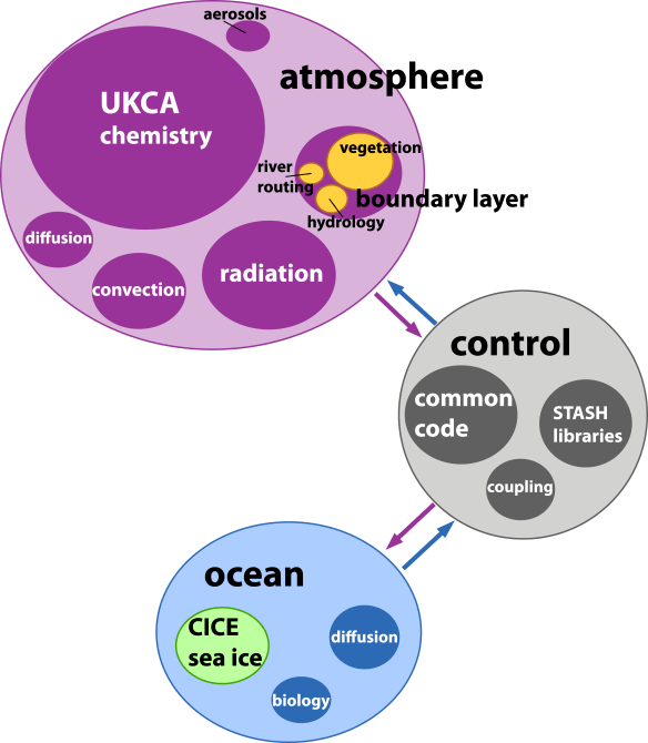
HadGEM2-ES
I will post future diagrams as they become available. We think the main use of these diagrams will be as communication tools between scientists, so they are free to use with attribution.

Just a few more weeks of classes, then I can enjoy some full-time research. Now that I’ve had a taste of being a proper scientist, it’s hard to go back!

A Vast Machine

I read Paul Edward’s A Vast Machine this summer while working with Steve Easterbrook. It was highly relevant to my research, but I would recommend it to anyone interested in climate change or mathematical modelling. Think The Discovery of Global Warming, but more specialized.

Much of the public seems to perceive observational data as superior to scientific models. The U.S. government has even attempted to mandate that research institutions focus on data above models, as if it is somehow more trustworthy. This is not the case. Data can have just as many problems as models, and when the two disagree, either could be wrong. For example, in a high school physics lab, I once calculated the acceleration due to gravity to be about 30 m/s2. There was nothing wrong with Newton’s Laws of Motion – our instrumentation was just faulty.

Additionally, data and models are inextricably linked. In meteorology, GCMs produce forecasts from observational data, but that same data from surface stations was fed through a series of algorithms – a model for interpolation – to make it cover an entire region. “Without models, there are no data,” Edwards proclaims, and he makes a convincing case.

The majority of the book discussed the history of climate modelling, from the 1800s until today. There was Arrhenius, followed by Angstrom who seemed to discredit the entire greenhouse theory, which was not revived until Callendar came along in the 1930s with a better spectroscope. There was the question of the ice ages, and the mistaken perception that forcing from CO2 and forcing from orbital changes (the Milankovitch model) were mutually exclusive.

For decades, those who studied the atmosphere were split into three groups, with three different strategies. Forecasters needed speed in their predictions, so they used intuition and historical analogues rather than numerical methods. Theoretical meteorologists wanted to understand weather using physics, but numerical methods for solving differential equations didn’t exist yet, so nothing was actually calculated. Empiricists thought the system was too complex for any kind of theory, so they just described climate using statistics, and didn’t worry about large-scale explanations.

The three groups began to merge as the computer age dawned and large amounts of calculations became feasible. Punch-cards came first, speeding up numerical forecasting considerably, but not enough to make it practical. ENIAC, the first model on a digital computer, allowed simulations to run as fast as real time (today the model can run on a phone, and 24 hours are simulated in less than a second).

Before long, theoretical meteorologists “inherited” the field of climatology. Large research institutions, such as NCAR, formed in an attempt to pool computing resources. With incredibly simplistic models and primitive computers (2-3 KB storage), the physicists were able to generate simulations that looked somewhat like the real world: Hadley cells, trade winds, and so on.

There were three main fronts for progress in atmospheric modelling: better numerical methods, which decreased errors from approximation; higher resolution models with more gridpoints; and higher complexity, including more physical processes. As well as forecast GCMs, which are initialized with observations and run at maximum resolution for about a week of simulated time, scientists developed climate GCMs. These didn’t use any observational data at all; instead, the “spin-up” process fed known forcings into a static Earth, started the planet spinning, and waited until it settled down into a complex climate and circulation that looked a lot like the real world. There was still tension between empiricism and theory in models, as some factors were parameterized rather than being included in the spin-up.

The Cold War, despite what it did to international relations, brought tremendous benefits to atmospheric science. Much of our understanding of the atmosphere and the observation infrastructure traces back to this period, when governments were monitoring nuclear fallout, spying on enemy countries with satellites, and considering small-scale geoengineering as warfare.

I appreciated how up-to-date this book was, as it discussed AR4, the MSU “satellites show cooling!” controversy, Watt’s Up With That, and the Republican anti-science movement. In particular, Edwards emphasized the distinction between skepticism for scientific purposes and skepticism for political purposes. “Does this mean we should pay no attention to alternative explanations or stop checking the data?” he writes. “As a matter of science, no…As a matter of policy, yes.”

Another passage beautifully sums up the entire narrative: “Like data about the climate’s past, model predictions of its future shimmer. Climate knowledge is probabilistic. You will never get a single definitive picture, either of exactly how much the climate has already changed or of how much it will change in the future. What you will get, instead, is a range. What the range tells you is that “no change at all” is simply not in the cards, and that something closer to the high end of the range – a climate catastrophe – looks all the more likely as time goes on.”

MPI Problem?

Now that my poster is finished, I am taking one last crack at getting CESM to run. Last time I wrote, I mentioned that the model execution was failing without giving any error messages (except the occasional “Segmentation fault”).

Michael Tobis thought that the problem had to do with mpiexec, so today I tried something new. I uninstalled mpich2 and replaced it with openmpi which I had built manually (as opposed to using apt-get). Now, when the model fails, the ccsm.log file actually says something:

mpiexec noticed that process rank 0 with PID 1846 on node computer name exited on signal 11 (Segmentation fault).
15 total processes killed (some possibly by mpiexec during cleanup)

Perhaps the problem is still with MPI. It seems unlikely that the segfault is due to a problem with the code itself (eg an undeclared variable), seeing as this version has been tested and used by NCAR. Maybe gcc is the issue, and I should play around with some compiler flags? Any suggestions would be welcome.

Wrapping Up

My summer job as a research student of Steve Easterbrook is nearing an end. All of a sudden, I only have a few days left, and the weather is (thankfully) cooling down as autumn approaches. It feels like just a few weeks ago that this summer was beginning!

Over the past three months, I examined seven different GCMs from Canada, the United States, and Europe. Based on the source code, documentation, and correspondence with scientists, I uncovered the underlying architecture of each model. This was represented in a set of diagrams. You can view full-sized versions here:

The component bubbles are to scale (based on the size of the code base) within each model, but not between models. The size and complexity of each GCM varies greatly, as can be seen below. UVic is by far the least complex model – it is arguably closer to an EMIC than a full GCM.

I came across many insights while comparing GCM architectures, regarding how modular components are, how extensively the coupler is used, and how complexity is distributed between components. I wrote some of these observations up into the poster I presented last week to the computer science department. My references can be seen here.

A big thanks to the scientists who answered questions about their work developing GCMs: Gavin Schmidt (Model E); Michael Eby (UVic); Tim Johns (HadGEM3); Arnaud Caubel, Marie-Alice Foujols, and Anne Cozic (IPSL); and Gary Strand (CESM). Additionally, Michael Eby from the University of Victoria was instrumental in improving the diagram design.

Although the summer is nearly over, our research certainly isn’t. I have started writing a more in-depth paper that Steve and I plan to develop during the year. We are also hoping to present our work at the upcoming AGU Fall Meeting, if our abstract gets accepted. Beyond this project, we are also looking at a potential experiment to run on CESM.

I guess I am sort of a scientist now. The line between “student” and “scientist” is blurry. I am taking classes, but also writing papers. Where does one end and the other begin? Regardless of where I am on the spectrum, I think I’m moving in the right direction. If this is what Doing Science means – investigating whatever little path interests me – I’m certainly enjoying it.

Progress?

I have made slight headway regarding my installation of CESM. It still isn’t running, but now it’s not running for a different reason than previously! Progress!

It appears that, at some point while porting, I mangled the scripts/ccsm_utils/Machines/mkbatch.kate file for my machine such that the actual call to launch the model wasn’t getting copied from mkbatch.kate to test.kate.run. A bit of trial and error fixed that problem.

I finally got Torque working. The only reason that jobs were getting stuck in the queue was that I didn’t start the pbs_sched daemon! It turns out that qsub isn’t related to the problems I was having, and isn’t necessary to run the model, but it’s nice to have it working just in case I need it in the future.

So, with the relevant call in test.kate.run as

mpiexec -n 16 ./ccsm.exe >&! ccsm.log.$LID

the command line output is

Wed July 6 11:02:33 EDT 2011 -- CSM EXECUTION BEGINS HERE
Wed July 6 11:02:34 EDT 2011 -- CSM EXECUTION HAS FINISHED
ls: No match.
Model did not complete - no cpl.log file present - exiting

The only log file created is ccsm.log, and it is completely empty.

I have MPICH2 installed, the command mpiexec seems to work fine, and I have mpd running. Regardless, I tried taking out mpiexec and calling the executable directly in test.kate.run:

./ccsm.exe >&! ccsm.log.$LID

The command line output becomes

Wed July 6 11:02:33 EDT 2011 -- CSM EXECUTION BEGINS HERE
Segmentation fault.
Wed July 6 11:02:34 EDT 2011 -- CSM EXECUTION HAS FINISHED
ls: No match.
Model did not complete - no cpl.log file present - exiting

Again, ccsm.log is empty, and there seems to be no trace of why the model is failing to launch beyond Segmentation fault. The CESM guide recommends setting the stack size to unlimited, which I did to no avail. Submitting test.kate.run using qsub produces the same messages, but in the output and error files, rather than the terminal.

Thoughts?

Modularity

I’ve now taken a look at the code and structure of four different climate models: Model E, CESM, UVic ESCM, and the Met Office Unified Model (which contains all the Hadley models). I’m noticing all sorts of similarities and differences, many of which I didn’t expect.

For example, I didn’t anticipate any overlap in climate model components. I thought that every modelling group would build their own ocean, their own atmosphere, and so on, from scratch. In fact, what I think of as a “model” – a self-contained, independent piece of software – applies to components more accurately than it does to an Earth system model. The latter is more accurately described as a collection of models, each representing one piece of the climate system. Each modelling group has a different collection of models, but not every one of these models is unique to their lab.

Ocean models are a particularly good example. The Modular Ocean Model (MOM) is built by GFDL, but it’s also used in NASA’s Model E and the UVic Earth System Climate Model. Another popular ocean model is the Nucleus for European Modelling of the Ocean (NEMO, what a great acronym) which is used by the newer Hadley climate models, as well as the IPSL model from France (which is sitting on my desktop as my next project!)

Aside: Speaking of clever acronyms, I don’t know what the folks at NCAR were thinking when they created the Single Column Atmosphere Model. Really, how did they not see their mistake? And why haven’t Marc Morano et al latched onto this acronym and spread it all over the web by now?

In most cases, an Earth system model has a unique architecture to fit all the component models together – a different coupling process. However, with the rise of standard interfaces like the Earth System Modeling Framework, even couplers can be reused between modelling groups. For example, the Hadley Centre and IPSL both use the OASIS coupler.

There are benefits and drawbacks to the rising overlap and “modularity” of Earth system models. One could argue that it makes the models less independent. If they all agree closely, how much of that agreement is due to their physical grounding in reality, and how much is due to the fact that they all use a lot of the same code? However, modularity is clearly a more efficient process for model development. It allows larger communities of scientists from each sub-discipline of Earth system modelling to form, and – in the case of MOM and NEMO – make two or three really good ocean models, instead of a dozen mediocre ones. Concentrating our effort, and reducing unnecessary duplication of code, makes modularity an attractive strategy, if an imperfect one.

The least modular of all the Earth system models I’ve looked at is Model E. The documentation mentions different components for the atmosphere, sea ice, and so on, but these components aren’t separated into subdirectories, and the lines between them are blurry. Nearly all the fortran files sit in the same directory, “model”,  and some of them deal with two or more components. For example, how would you categorize a file that calculates surface-atmosphere fluxes? Even where Model E uses code from other institutions, such as the MOM ocean model, it’s usually adapted and integrated into their own files, rather than in a separate directory.

The most modular Earth system model is probably the Met Office Unified Model. They don’t appear to have adapted NEMO, CICE (the sea ice model from NCAR) and OASIS at all – in fact, they’re not present in the code repository they gave us. I was a bit confused when I discovered that their “ocean” directory, left over from the years when they wrote their own ocean code, was now completely empty! Encapsulation to the point where a component model can be stored completely externally to the structural code was unexpected.

An interesting example of the challenges of modularity appears in sea ice. Do you create a separate, independent sea ice component, like CESM did? Do you consider it part of the ocean, like NEMO? Or do you lump in lake ice along with sea ice and subsequently allow the component to float between the surface and the ocean, like Model E?

The real world isn’t modular. There are no clear boundaries between components on the physical Earth. But then, there’s only one physical Earth, whereas there are many virtual Earths in the form of climate modelling, and limited resources for developing the code in each component. In this spectrum of interconnection and encapsulation, is one end or the other our best bet? Or is there a healthy balance somewhere in the middle?

Working Away

The shape of my summer research is slowly becoming clearer. Basically, I’ll be writing a document comparing the architecture of different climate models. This, of course, involves getting access to the source code. Building on Steve’s list, here are my experiences:

NCAR, Community Earth System Model (CESM): Password-protected, but you can get access within an hour. After a quick registration, you’ll receive an automated email with a username and password. This login information gives you access to their Subversion repository. Registration links and further information are available here, under “Acquiring the CESM1.0 Release Code”.

University of Victoria, Earth System Climate Model (ESCM): Links to the source code can be found on this page, but they’re password-protected. You can request an account by sending an email – follow the link for more information.

Geophysical Fluid Dynamics Laboratory (GFDL), CM 2.1: Slightly more complicated. Create an account for their Gforge repository, which is an automated process. Then, request access to the MOM4P1 project – apparently CM 2.1 is included within that. Apparently, the server grants you request to a project, so it sounds automatic – but the only emails I’ve received from the server regard some kind of GFDL mailing list, and don’t mention the project request. I will wait and see.
Update (July 20): It looks like I got access to the project right after I requested it – I just never received an email!

Max Planck Institute (MPI), COSMOS: Code access involves signing a licence agreement, faxing it to Germany, and waiting for it to be approved and signed by MPI. The agreement is not very restrictive, though – it deals mainly with version control, documenting changes to the code, etc.

UK Met Office, Hadley Centre Coupled Model version 3 (HadCM3): Our lab already has a copy of the code for HadCM3, so I’m not really sure what the process is to get access, but apparently it involved a lot of government paperwork.

Institut Pierre Simon Laplace (IPSL), CM5: This one tripped me up for a while, largely because the user guide is difficult to find, and written in French. Google Translate helped me out there, but it also attempted to “translate” their command line samples! Make sure that you have ksh installed, too – it’s quick to fix, but I didn’t realize it right away. Some of the components for IPSLCM5 are open access, but others are password-protected. Follow the user guide’s instructions for who to email to request access.

Model E: This was the easiest of all. From the GISS website, you can access all the source code without any registration. They offer a frozen AR4 version, as well as nightly snapshots of the work-in-process for AR5 (frozen AR5 version soon to come). There is also a wealth of documentation on this site, such as an installation guide and a description of the model.

I’ve taken a look at the structural code for Model E, which is mostly contained in the file MODELE.f. The code is very clear and well commented, and the online documentation helped me out too. After drawing a lot of complicated diagrams with arrows and lists, I feel that I have a decent understanding of the Model E architecture.

Reading code can become monotonous, though, and every now and then I feel like a little computer trouble to keep things interesting. For that reason, I’m continuing to chip away at building and running two models, Model E and CESM. See my previous post for how this process started.

<TECHNICAL COMPUTER STUFF> (Feel free to skip ahead…)

I was still having trouble viewing the Model E output (only one file worked on Panoply, the rest created an empty map) so I emailed some of the lab’s contacts at NASA. They suggested I install CDAT, a process which nearly broke Ubuntu (haven’t we all been there?) Basically, because it’s an older program, it thought the newest version of Python was 2.5 – which it subsequently installed and set as the default in /usr/bin. Since I had Python 2.6 installed, and the versions are apparently very not-backwards-compatible, every program that depended on Python (i.e. almost everything on Ubuntu) stopped working. Our IT contact managed to set 2.6 back as the default, but I’m not about to try my hand at CDAT again…

I have moved forward very slightly on CESM. I’ve managed to build the model, but upon calling test.<machine name>.run, I get rather an odd error:

./Tools/ccsm_getenv: line 9: syntax error near unexpected token '('
./Tools/ccsm_getenv: line 9: 'foreach i (env_case.xml env_run.xml env_conf.xml env_build.xml env_mach_pes.xml)'

Now, I’m pretty new at shell scripting, but I can’t see the syntax error there – and wouldn’t syntax errors appear at compile-time, rather than run-time?

A post by Michael Tobis, who had a similar error, suggested that the issue had to do with qsub. Unfortunately, that meant I had to actually use qsub – I had previously given up trying to configure Torque to run on a single machine rather than many. I gave the installation another go, and now I can get scripts into the queue, but they never start running – their status stays as “Q” even if I leave the computer alone for an hour. Since the machine has a dual-core processor, I can’t see why it couldn’t run both a server and a node at once, but it doesn’t seem to be working for me.

</TECHNICAL COMPUTER STUFF>

Before I started this job, climate models seemed analogous to Antarctica – a distant, mysterious, complex system that I wanted to visit, but didn’t know how to get to. In fact, they’re far more accessible than Antarctica. More on the scale of a complicated bus trip across town, perhaps?

They are not perfect pieces of software, and they’re not very user friendly. However, all the struggles of installation pay off when you finally get some output, and open it up, and see realistic data representing the very same planet you’re sitting on! Even just reading the code for different models shows you many different ways to look at the same system – for example, is sea ice a realm of its own, or is it a subset of the ocean? In the real world the lines are blurry, but computation requires us to make clear divisions.

The code can be unintelligible (lndmaxjovrdmdni) or familiar (“The Stefan-Boltzmann constant! Finally I recognize something!”) or even entertaining (a seemingly random identification string, dozens of characters long, followed by the comment if you edit this you will get what you deserve). When you get tied up in the code, though, it’s easy to miss the bigger picture: the incredible fact that we can use the sterile, binary practice of computation to represent a system as messy and mysterious as the whole planet. Isn’t that something worth sitting and marveling over?

Climate Models on Ubuntu

Part 1: Model E

I felt a bit over my head attempting to port CESM, so I asked a grad student, who had done his Master’s on climate modelling, for help. He looked at the documentation, scratched his head, and suggested I start with NASA’s Model E instead, because it was easier to install. And was it ever! We had it up and running within an hour or so. It was probably so much easier because Model E comes with gfortran support, while CESM only has scripts written for commercial compilers like Intel or PGI.

Strangely, when using Model E, no matter what dates the rundeck sets for the simulation start and end, the subsequently generated I file always has December 1, 1949 as the start date and December 2, 1949 as the end date. We edited the I files after they were created, which seemed to fix the problem, but it was still kind of weird.

I set up Model E to run a ten-year simulation with fixed atmospheric concentration (really, I just picked a rundeck at random) over the weekend. It took it about 3 days to complete, so just over 7 hours per year of simulation time…not bad for a 32-bit desktop!

However, I’m having some weird problems with the output – after configuring the model to output files in NetCDF format and opening them in Panoply, only the file with all the sea ice variables worked. All the others either gave a blank map (array full of N/A’s) or threw errors when Panoply tried to read them. Perhaps the model isn’t enjoying having the I file edited?

Part 2: CESM

After exploring Model E, I felt like trying my hand at CESM again. Steve managed to port it onto his Macbook last year, and took detailed notes. Editing the scripts didn’t seem so ominous this time!

The CESM code can be downloaded using Subversion (instructions here) after a quick registration. Using the Ubuntu Software Center, I downloaded some necessary packages: libnetcdf-dev, mpich2, and torque-scheduler. I already had gfortran, which is sort of essential.

I used the Porting via user defined machine files method to configure the model for my machine, using the Hadley scripts as a starting point. Variables for the config_machines.xml are explained in Appendix D through H of the user’s guide (links in chapter 7). Mostly, you’re just pointing to folders where you want to store data and files. Here are a few exceptions:

  • DOUT_L_HTAR: I stuck with "TRUE", as that was the default.
  • CCSM_CPRNC: this tool already exists in the CESM source code, in /models/atm/cam/tools/cprnc.
  • BATCHQUERY and BATCHSUBMIT: the Hadley entry had “qstat” and “qsub”, respectively, so I Googled these terms to find out which batch submission software they referred to (Torque, which is freely available in the torque-scheduler package) and downloaded it so I could keep the commands the same!
  • GMAKE_J: this determines how many processors to commit to a certain task, and I wasn’t sure how many this machine had, so I just put “1”.
  • MAX_TASKS_PER_NODE: I chose "8", which the user’s guide had mentioned as an example.
  • MPISERIAL_SUPPORT: the default is “FALSE”.

The only file that I really needed to edit was Macros.<machine name>. The env_machopts.<machine name> file ended up being empty for me. I spent a while confused by the modules declarations, which turned out to refer to the Environment Modules software. Once I realized that, for this software to be helpful, I would have to write five or six modulefiles in a language I didn’t know, I decided that it probably wasn’t worth the effort, and took these declarations out. I left mkbatch.<machine name> alone, except for the first line which sets the machine, and then turned my attention to Macros.

“Getting this to work will be an iterative process”, the user’s guide says, and it certainly was (and still is). It’s never a good sign when the installation guide reminds you to be patient! Here is the sequence of each iteration:

  1. Edit the Macros file as best I can.
  2. Open up the terminal, cd to cesm1_0/scripts, and create a new case as follows: ./create_newcase -case test -res f19_g16 -compset X -mach <machine name>
  3. If this works, cd to test, and run configure: ./configure -case
  4. If all is well, try to build the case: ./test.<machine name>.build
  5. See where it fails and read the build log file it refers to for ideas as to what went wrong. Search on Google for what certain errors mean. Do some other work for a while, to let the ideas simmer.
  6. Set up for the next case: ./test.<machine name>.clean_build , cd .., and rm -rf test. This clears out old files so you can safely build a new case with the same name.
  7. See step 1.

I wasn’t really sure what the program paths were, as I couldn’t find a nicely contained folder for each one (like Windows has in “Program Files”), but I soon stumbled upon a nice little trick: look up the package on Ubuntu Package Manager, and click on “list of files” under the Download section. That should tell you what path the program used as its root.

I also discovered that setting FC and CC to gfortran and gcc, respectively, in the Macros file will throw errors. Instead, leave the variables as mpif90 and mpicc, which are linked to the GNU compilers. For example, when I type mpif90 in the terminal, the result is gfortran: no input files, just as if I had typed gfortran. For some reason, though, the errors go away.

As soon as I made it past building the mct and pio libraries, the build logs for each component (eg atm, ice) started saying gmake: command not found. This is one of the pitfalls of Ubuntu: it uses the command make for the same program that basically every other Unix-based OS calls gmake. So I needed to find and edit all the scripts that called gmake, or generated other scripts that called it, and so on. “There must be a way to automate this,” I thought, and from this article I found out how. In the terminal, cd to the CESM source code folder, and type the following:

grep -lr -e 'gmake' * | xargs sed -i 's/gmake/make/g'

You should only have to do this once. It’s case sensitive, so it will leave the xml variable GMAKE_J alone.

Then I turned my attention to compiler flags, which Steve chronicled quite well in his notes (see link above). I made most of the same changes that he did, except I didn’t need to change -DLINUX to -DDarwin. However, I needed some more compiler flags still. In the terminal, man gfortran brings up a list of all the options for gfortran, which was helpful.

The ccsm build log had hundreds of undefined reference errors as soon as it started to compile fortran. The way I understand it, many of the fortran files reference each other, but gfortran likes to append underscores to user-defined variables, and then it can’t find the file the variable is referencing! You can suppress this using the flag -fno-underscoring.

Now I am stuck on a new error. It looks like the ccsm script is almost reaching the end, as it’s using ld, the gcc linking mechanism, to tie all the files together. Then the build log says:

/usr/bin/ld: seq_domain_mct.o(.debug_info+0x1c32): unresolvable R_386_32 relocation against symbol 'mpi_fortran_argv_null'
/usr/bin/ld: final link failed: Nonrepresentable section on output
collect2: ld returned 1 exit status

I’m having trouble finding articles on the internet about similar errors, and the gcc and ld manpages are so long that trying every compiler flag isn’t really an option. Any ideas?

Update: Fixed it! In scripts/ccsm_utils/Build/Makefile, I changed LD := $(F90) to LD := gcc -shared. The build was finally successful! Now off to try and run it…

The good thing is that, since I re-started this project a few days ago, I haven’t spent very long stuck on any one error. I’m constantly having problems, but I move through them pretty quickly! In the meantime, I’m learning a lot about the model and how it fits everything together during installation. I’ve also come a long way with Linux programming in general. Considering that when I first installed Ubuntu a few months ago, and sheepishly called my friend to ask where to find the command line, I’m quite proud of my progress!

I hope this article will help future Ubuntu users install CESM, as it seems to have a few quirks that even Mac OS X doesn’t experience (eg make vs gmake). For the rest of you, apologies if I have bored you to tears!

Tornadoes and Climate Change

Cross-posted from NextGen Journal

It has been a bad season for tornadoes in the United States. In fact, this April shattered the previous record for the most tornadoes ever. Even though the count isn’t finalized yet, nobody doubts that it will come out on top:

In a warming world, many questions are common, and quite reasonable. Is this a sign of climate change? Will we experience more, or stronger, tornadoes as the planet warms further?

In fact, these are very difficult questions to answer. First of all, attributing a specific weather event, or even a series of weather events, to a change in the climate is extremely difficult. Scientists can do statistical analysis to estimate the probability of the event with and without the extra energy available in a warming world, but this kind of study takes years. Even so, nobody can say for certain whether an event wasn’t just a fluke. The recent tornadoes very well might have been caused by climate change, but they also might have happened anyway.

Will tornadoes become more common in the future, as global warming progresses? Tornado formation is complicated, and forecasting them requires an awful lot of calculations. Many processes in the climate system are this way, so scientists simulate them using computer models, which can do detailed calculations at an increasingly impressive speed.

However, individual tornadoes are relatively small compared to other kinds of storms, such as hurricanes or regular rainstorms. They are, in fact, smaller than a single square in the highest-resolution climate models around today. Therefore, it’s just not possible to directly project them using mathematical models.

However, we can project the conditions necessary for tornadoes to form. They don’t always lead to a tornado, but they make one more likely. Two main factors exist: high wind shear and high convective available potential energy (CAPE). Climate change is making the atmosphere warmer, and increasing specific humidity (but not relative humidity): both of these contribute to CAPE, so that factor will increase the likelihood of conditions favourable to tornadoes. However, climate change warms the poles faster than the equator, which will decrease the temperature difference between them, subsequently lowering wind shear. That will make tornadoes less likely (Diffenbaugh et al, 2008). Which factor will win out? Is there another factor involved that climate change could impact? Will we get more tornadoes in some areas and less in others? Will we get weaker tornadoes or stronger tornadoes? It’s very difficult to tell.

In 2007, NASA scientists used a climate model to project changes in severe storms, including tornadoes. (Remember, even though an individual tornado can’t be represented on a model, the conditions likely to cause a tornado can.) They predicted that the future will bring fewer storms overall, but that the ones that do form will be stronger. A plausible solution to the question, although not a very comforting one.

With uncertain knowledge, how should we approach this issue? Should we focus on the comforting possibility that the devastation in the United States might have nothing to do with our species’ actions? Or should we acknowledge that we might bear responsibility? Dr. Kevin Trenberth, a top climate scientist at the National Center for Atmospheric Research (NCAR), thinks that ignoring this possibility until it’s proven is a bad idea. “It’s irresponsible not to mention climate change,” he writes.

Learning Experiences

I apologize for my brief hiatus – it’s been almost two weeks since I’ve posted. I have been very busy recently, but for a very exciting reason: I got a job as a summer student of Dr. Steve Easterbrook! You can read more about Steve and his research on his faculty page and blog.

This job required me to move cities for the summer, so my mind has been consumed with thoughts such as “Where am I and how do I get home from this grocery store?” rather than “What am I going to write a post about this week?” However, I have had a few days on the job now, and as Steve encourages all of his students to blog about their research, I will use this outlet to periodically organize my thoughts.

I will be doing some sort of research project about climate modelling this summer – we’re not yet sure exactly what, so I am starting by taking a look at the code for some GCMs. The NCAR Community Earth System Model is one of the easiest to access, as it is largely an open source project. I’ve only read through a small piece of their atmosphere component, but I’ve already seen more physics calculations in one place than ever before.

I quickly learned that trying to understand every line of the code is a silly goal, as much as I may want to. Instead, I’m trying to get a broader picture of what the programs do. It’s really neat to have my knowledge about different subjects converge so completely. Multi-dimensional arrays, which I have previously only used to program games of Sudoku and tic-tac-toe, are now being used to represent the entire globe. Electric potential, a property I last studied in the circuitry unit of high school physics, somehow impacts atmospheric chemistry. The polar regions, which I was previously fascinated with mainly for their wildlife, also present interesting mathematical boundary cases for a climate model.

It’s also interesting to see how the collaborative nature of CESM, written by many different authors and designed for many different purposes, impacts its code. Some of the modules have nearly a thousand lines of code, and some have only a few dozen – it all depends on the programming style of the various authors. The commenting ranges from extensive to nonexistent. Every now and then one of the files will be written in an older version of Fortran, where EVERYTHING IS IN UPPER CASE.

I am bewildered by most of the variable names. They seem to be collections of abbreviations I’m not familiar with. Some examples are “mxsedfac”, “lndmaxjovrdmdni”, “fxdd”, and “vsc_knm_atm”.

When we get a Linux machine set up (I have heard too many horror stories to attempt a dual-boot with Windows) I am hoping to get a basic CESM simulation running, as well as EdGCM (this could theoretically run on my laptop, but I prefer to bring that home with me each evening, and the simulation will probably take over a day).

I am also doing some background reading on the topic of climate modelling, including this book, which led me to the story of PHONIAC. The first weather prediction done on a computer (the ENIAC machine) was recreated as a smartphone application, and ran approximately 3 million times faster. Unfortunately, I can’t find anyone with a smartphone that supports Java (argh, Apple!) so I haven’t been able to try it out.

I hope everyone is having a good summer so far. A more traditional article about tornadoes will be coming at the end of the week.