Breaching the Mainstream

It’s hard to overestimate the influence of John and Hank Green on the Internet, particularly among people my age. John (who writes books for teenagers) and Hank (who maintains the website EcoGeek and sings songs about particle physics) run a YouTube channel that celebrates nerdiness. This Internet community is now a huge part of pop culture among self-professed teenage nerds.

Hank’s new spin-off channel SciShow, which publishes videos about popular science topics, has only being going for a month but already has 90 000 subscribers and 1 million views. So I was very excited when Hank created this entertaining, polished, and wonderfully accurate video about climate change. He discusses sea level rise, anoxic events, and even the psychology of denial:

How much is most?

A growing body of research is showing that humans are likely causing more than 100% of global warming: without our influences on the climate, the planet would actually be cooling slightly.

In 2007, the Intergovernmental Panel on Climate Change published its fourth assessment report, internationally regarded as the most credible summary of climate science to date. It concluded that “most of the observed increase in global average temperatures since the mid-20th century is very likely due to the observed increase in anthropogenic greenhouse gas concentrations”.

A clear question remains: How much is “most”? 51%? 75%? 99%? At the time that the IPCC report was written, the answer was unclear. However, a new frontier of climate research has emerged since, and scientists are working hard to quantify the answer to this question.

I recently attended the 2011 American Geophysical Union Fall Meeting, a conference of over 20 000 scientists, many of whom study the climate system. This new area of research was a hot topic of discussion at AGU, and a phrase that came up many times was “more than 100%”.

That’s right, humans are probably causing more than 100% of observed global warming. That means that our influences are being offset by natural cooling factors. If we had never started burning fossil fuels, the world would be cooling slightly.

In the long term, oscillations of the Earth’s orbit show that, without human activity, we would be very slowly descending into a new ice age. There are other short-term cooling influences, though. Large volcanic eruptions, such as Mount Pinatubo in 1991, have thrown dust into the upper atmosphere where it blocks a small amount of sunlight. The sun, particularly in the last few years, has been less intense than usual, due to the 11-year sunspot cycle. We have also experienced several strong La Niña events in the Pacific Ocean, which move heat out of the atmosphere and into the ocean.

However, all of these cooling influences pale in comparison to the strength of the human-caused warming influences. The climate change communication project Skeptical Science recently summarized six scientific studies in this graphic:

Most of the studies estimated that humans caused over 100% of the warming since 1950, and all six put the number over 98%. Additionally, most of the studies find natural influences to be in the direction of cooling, and all six show that number to be close to zero.

If you are interested in the methodologies and uncertainty ranges of these six studies, Skeptical Science goes into more detail, and also provides links to the original journal articles.

To summarize, the perception that humans are accelerating a natural process of warming is false. We have created this problem entirely on our own. Luckily, that means we have the power to stop the problem in its tracks. We are in control, and we choose what happens in the future.

Winter in the Woods

Do not burn yourself out. Be as I am – a reluctant enthusiast… a part time crusader, a half-hearted fanatic. Save the other half of yourselves and your lives for pleasure and adventure. It is not enough to fight for the land; it is even more important to enjoy it. While you can. While it is still there. So get out there and mess around with your friends, ramble out yonder and explore the forests, encounter the grizz, climb the mountains. Run the rivers, breathe deep of that yet sweet and lucid air, sit quietly for a while and contemplate the precious stillness, that lovely, mysterious and awesome space. Enjoy yourselves, keep your brain in your head and your head firmly attached to your body, the body active and alive, and I promise you this much: I promise you this one sweet victory over our enemies, over those deskbound people with their hearts in a safe deposit box and their eyes hypnotized by desk calculators. I promise you this: you will outlive the bastards.

So writes Edward Abbey, in a passage that Ken sent to me nearly two years ago. The quote is now stuck to my fridge, and I abide by it as best I can.

It’s pretty easy to find areas of untouched forest within my city. Living in a floodplain, it’s only practical to leave natural vegetation growing around the rivers – it acts as a natural sponge when the water rises. In the warmer months, hiking in the woods is convenient, particularly because I can bike to the edge of the river. But in the winter, it’s not so easy. The past few months have consistently been about 10 C above normal, though, and today I found a shortcut that made the trip to the woods walkable.

The aspen parkland in winter is strange. Most wildlife travel south or begin hibernating by early October, and no evergreen species grow here naturally. As you walk through the naked branches, it’s easy to think of the woods as desolate. But if you slow down, pay attention, and look around more carefully, you see signs of life in the distance:

Black-capped Chickadee

White-tailed Deer

If you stand still and do your best to look non-threatening, some of the more curious animals might come for a closer inspection:

If you imitate a bird's call well enough, it will come right up to you

A mother deer and her fawn, probably about eight months old

The species that live here year-round are some of the most resilient on the continent. They have survived 40 above and 40 below, near-annual droughts and floods, and 150 years of colonization. The Prairies is a climate of extremes, and life has evolved to thrive in those extremes.

So maybe this isn’t the land I am fighting for – it will probably be able to handle whatever climate change throws at it – but it is the land I love regardless.

Happy Christmas to everyone, and please go out and enjoy the land you’re fighting for, as a gift to yourself.

What Happened At Durban?

Cross-posted from NextGen Journal

Following the COP17 talks in Durban, South Africa – the latest attempt to create a global deal to cut carbon emissions and solve global warming – world leaders claimed they had “made history”, calling the conference “a great success” that had “all the elements we were looking for”.

So what agreement did they all come to, that has them so proud? They agreed to figure out a deal by 2015. As James Hrynyshyn writes, it is “a roadmap to a unknown strategy that may or may not produce a plan that might combat climate change”.

Did I miss a meeting? Weren’t we supposed to figure out a deal by 2010, so it could come into force when the Kyoto Protocol expires in 2012? This unidentified future deal, if it even comes to pass, will not come into force until 2020 – that’s 8 years of unchecked global carbon emissions.

At COP15 in Copenhagen, countries agreed to limit global warming to 2 degrees Celsius. The German Advisory Council on Global Change crunched the numbers and discovered that the sooner we start reducing emissions, the easier it will be to attain this goal. This graph shows that if emissions peak in 2011 we have a “bunny slope” to ride, whereas if emissions peak in 2020 we have a “triple black diamond” that’s almost impossible, economically. (Thanks to Richard Sommerville for this analogy).

If we stay on the path that leaders agreed on in Durban, emissions will peak long after 2020 – in the best case scenario, they will only start slowing in 2020. If the triple black diamond looks steep, imagine a graph where emissions peak in 2030 or 2040 – it’s basically impossible to achieve our goal, no matter how high we tax carbon or how many wind turbines we build.

World leaders have committed our generation to a future where global warming spins out of our control. What is there to celebrate about that?

However, we shouldn’t throw our hands in the air and give up. 2 degrees is bad, but 4 degrees is worse, and 6 degrees is awful. There is never a point at which action is pointless, because the problem can always get worse if we ignore it.

The Software Architecture of Global Climate Models

Last week at AGU, I presented the results of the project Steve Easterbrook and I worked on this summer. Click the thumbnail on the left for a full size PDF. Also, you can download the updated versions of our software diagrams:

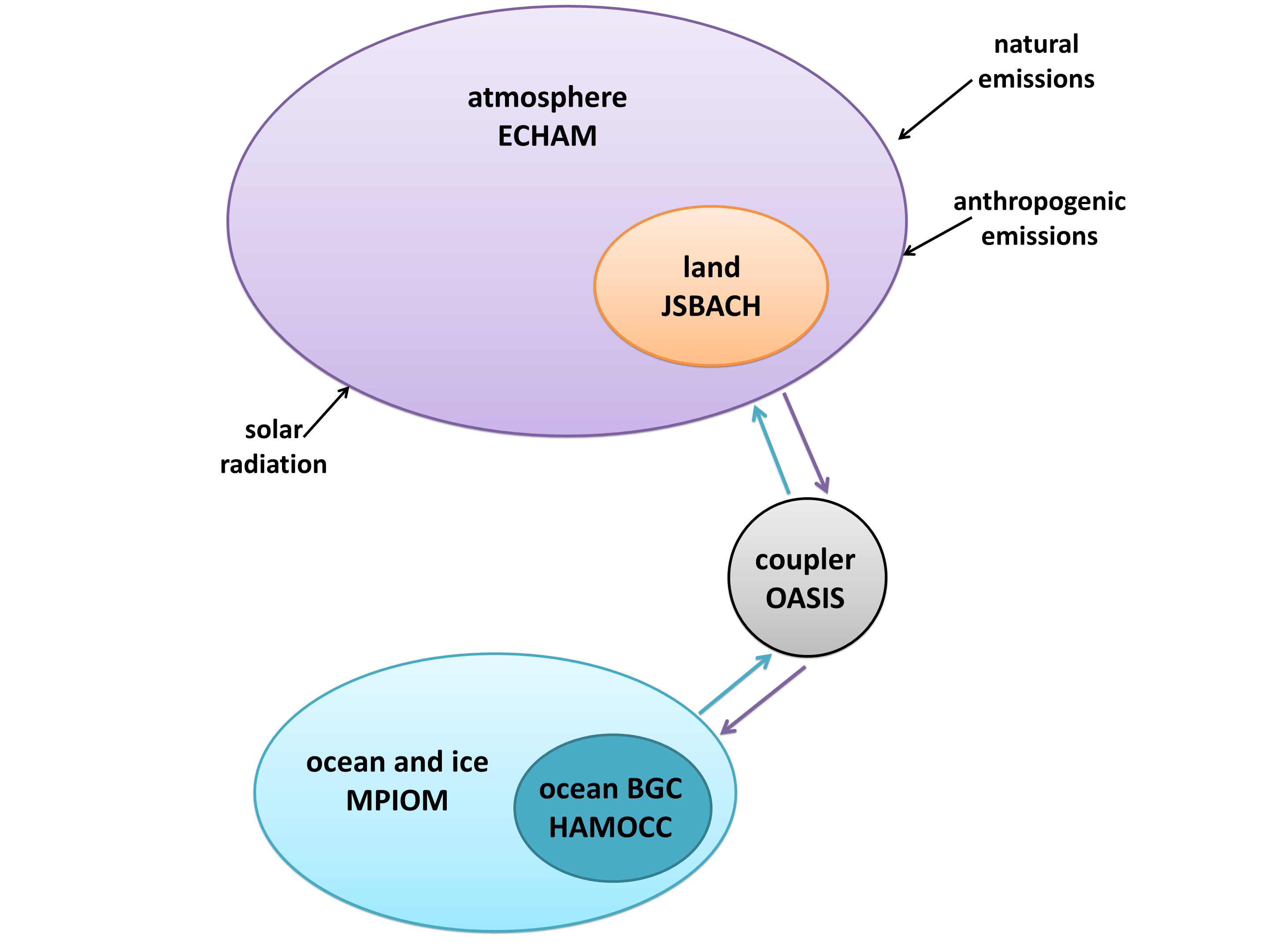
  • COSMOS (COmmunity earth System MOdelS) 1.2.1
  • Model E: Oct. 11, 2011 snapshot
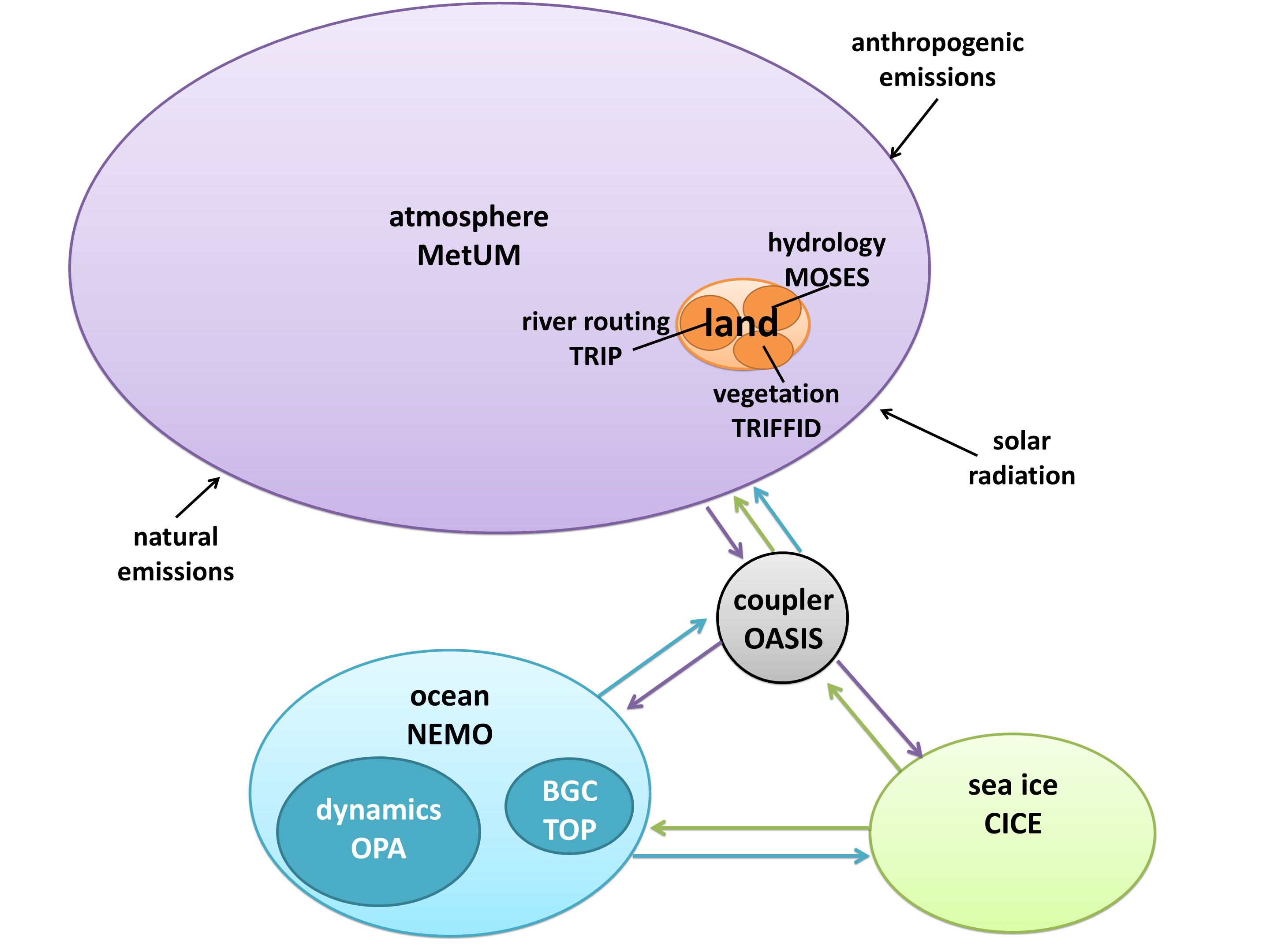
  • HadGEM3 (Hadley Centre Global Environmental Model, version 3): August 2009 snapshot
  • CESM (Community Earth System Model) 1.0.3
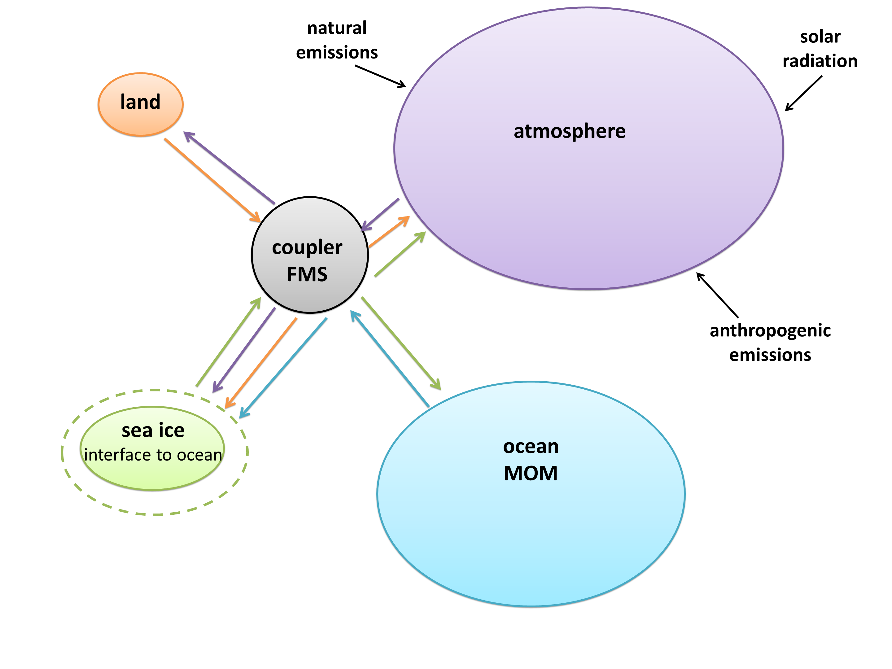
  • GFDL (Geophysical Fluid Dynamics Laboratory), Climate Model 2.1 coupled to MOM (Modular Ocean Model) 4.1
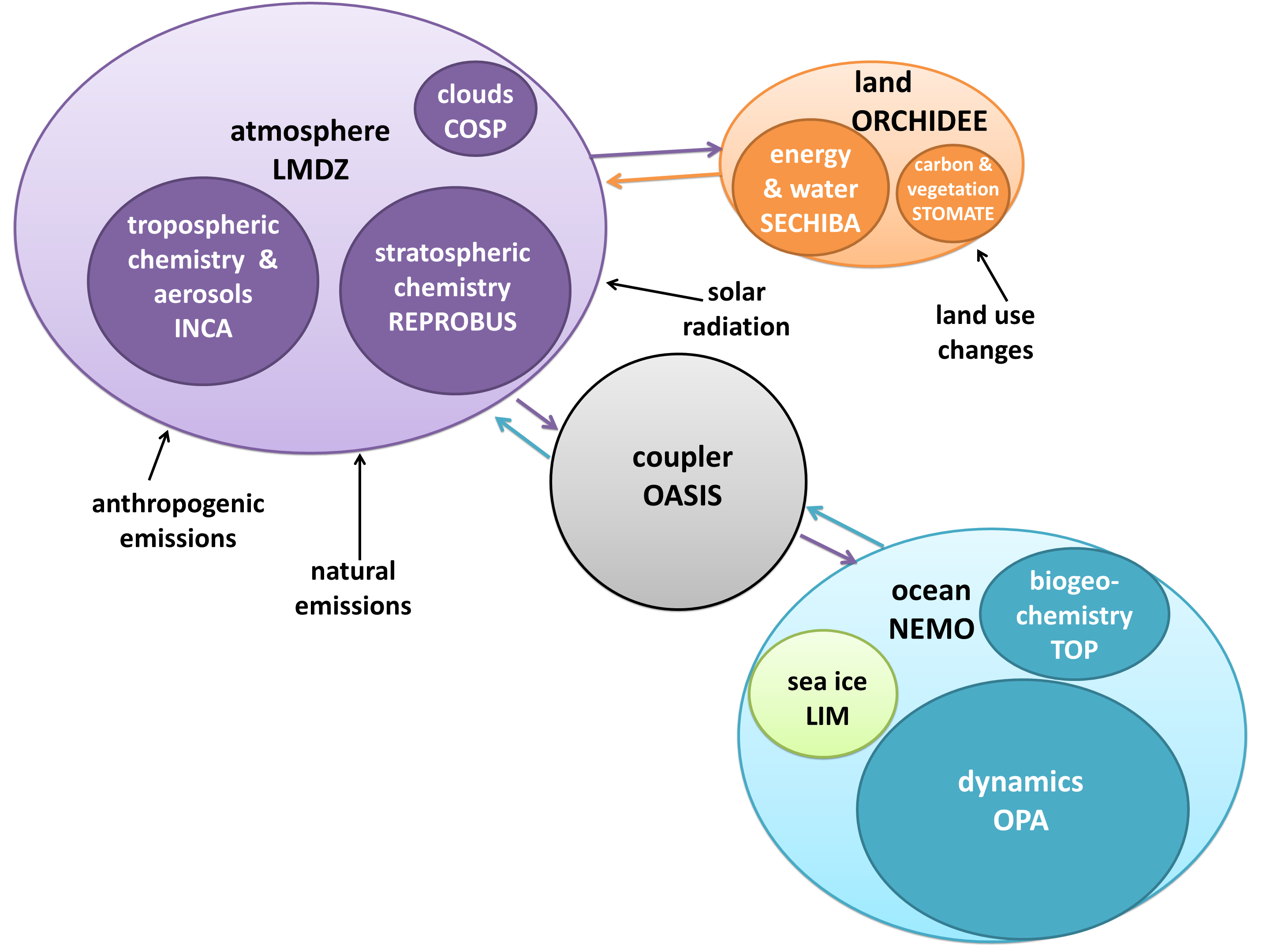
  • IPSL (Institut Pierre Simon Laplace), Climate Model 5A
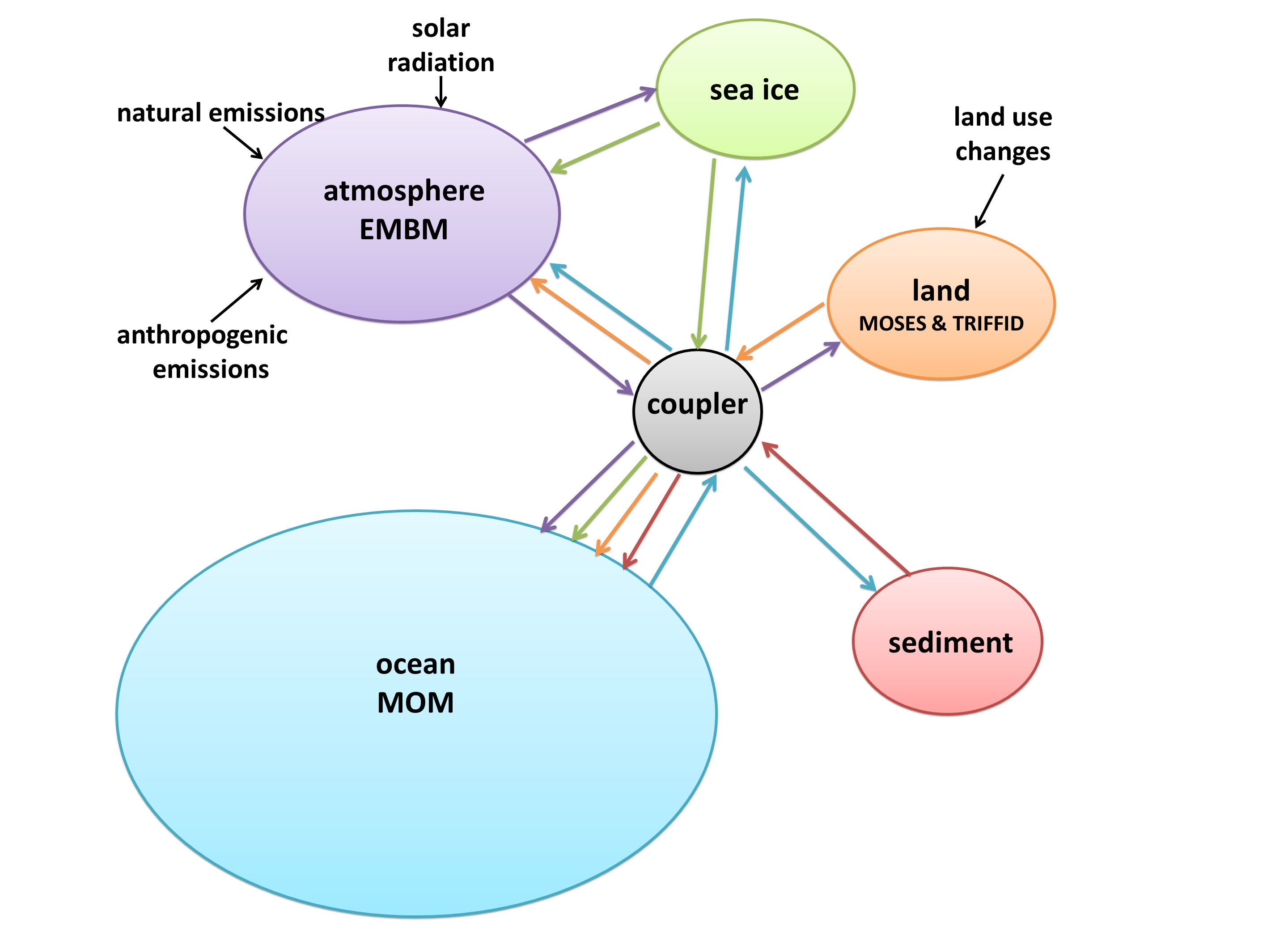
  • UVic ESCM (Earth System Climate Model) 2.9

And, since the most important part of poster sessions is the schpiel you give and the conversations you have, here is my schpiel:

Steve and I realized that while comparisons of the output of global climate models are very common (for example, CMIP5: Coupled Model Intercomparison Project Phase 5), nobody has really sat down and compared their software structure. We tried to fill this gap in research with a qualitative comparison study of seven models. Six of them are GCMs (General Circulation Models – the most complex climate simulations) in the CMIP5 ensemble; one, the UVic model, is not in CMIP because it’s really more of an EMIC (Earth System Model of Intermediate Complexity – simpler than a GCM). However, it’s one of the most complex EMICs, and contains a full GCM ocean, so we thought it would present an interesting boundary case. (Also, the code was easier to get access to than the corresponding GCM from Environment Canada. When we write this up into a paper we will probably use that model instead.)

I created a diagram of each model’s architecture. The area of each bubble is roughly proportional to the lines of code in that component, which we think is a pretty good proxy for complexity – a more complex model will have more subroutines and functions than a simple one. The bubbles are to scale within each model, but not between models, as the total lines of code in a model varies by about a factor of 10. A bit difficult to fit on a poster and still make everything readable! Fluxes from each component are represented by coloured arrows (the same colour as the bubble), and often pass through the coupler before reaching another component.

We examined the amount of encapsulation of components, which varies widely between models. CESM, on one end of the spectrum, isolates every component completely, particularly in the directory structure. Model E, on the other hand, places nearly all of its files in the same directory, and has a much higher level of integration between components. This is more difficult for a user to read, but it has benefits for data transfer.

While component encapsulation is attractive from a software engineering perspective, it poses problems because the real world is not so encapsulated. Perhaps the best example of this is sea ice. It floats on the ocean, its extent changing continuously. It breaks up into separate chunks and can form slush with the seawater. How do you split up ocean code and ice code? CESM keeps the two components completely separate, with a transient boundary between them. IPSL represents ice as an encapsulated sub-component of their ocean model, NEMO (Nucleus for European Modeling of the Ocean). COSMOS integrates both ocean and ice code together in MPI-OM (Max Planck Institute Ocean Model).

GFDL took a completely different, and rather innovative, approach. Sea ice in the GFDL model is an interface, a layer over the ocean with boolean flags in each cell indicating whether or not ice is present. All fluxes to and from the ocean must pass through the “sea ice”, even if they’re at the equator and the interface is empty.

Encapsulation requires code to tie components together, since the climate system is so interconnected. Every model has a coupler, which fulfills two main functions: controlling the main time-stepping loop, and passing data between components. Some models, such as CESM, use the coupler for every interaction. However, if two components have the same grid, no interpolation is necessary, so it’s often simpler just to pass them directly. Sometimes this means a component can be completely disconnected from the coupler, such as the land model in IPSL; other times it still uses the coupler for other interactions, such as the HadGEM3 arrangement with direct ocean-ice fluxes but coupler-controlled ocean-atmosphere and ice-atmosphere fluxes.

While it’s easy to see that some models are more complex than others, it’s also interesting to look at the distribution of complexity within a model. Often the bulk of the code is concentrated in one component, due to historical software development as well as the institution’s conscious goals. Most of the models are atmosphere-centric, since they were created in the 1970s when numerical weather prediction was the focus of the Earth system modelling community. Weather models require a very complex atmosphere but not a lot else, so atmospheric routines dominated the code. Over time, other components were added, but the atmosphere remained at the heart of the models. The most extreme example is HadGEM3, which actually uses the same atmosphere model for both weather prediction and climate simulations!

The UVic model is quite different. The University of Victoria is on the west coast of Canada, and does a lot of ocean studies, so the model began as a branch of the MOM ocean model from GFDL. The developers could have coupled it to a complex atmosphere model in an effort to mimic full GCMs, but they consciously chose not to. Atmospheric routines need very short time steps, so they eat up most of the run time, and make very long simulations not feasible. In an effort to keep their model fast, UVic created EMBM (Energy Moisture Balance Model), an extremely simple atmospheric model (for example, it doesn’t include dynamic precipitation – it simply rains as soon as a certain humidity is reached). Since the ocean is the primary moderator of climate over the long run, the UVic ESCM still outputs global long-term averages that match up nicely with GCM results.

Finally, CESM and Model E could not be described as “land-centric”, but land is definitely catching up – it’s even surpassed the ocean model in both cases! These two GCMs are cutting-edge in terms of carbon cycle feedbacks, which are primarily terrestrial, and likely very important in determining how much warming we can expect in the centuries to come. They are currently poorly understood and difficult to model, so they are a new frontier for Earth system modelling. Scientists are moving away from a binary atmosphere-ocean paradigm and towards a more comprehensive climate system representation.

I presented this work to some computer scientists in the summer, and many of them asked, “Why do you need so many models? Wouldn’t it be better to just have one really good one that everyone collaborated on?” It might be simpler from a software engineering perspective, but for the purposes of science, a variety of diverse models is actually better. It means you can pick and choose which model suits your experiment. Additionally, it increases our confidence in climate model output, because if dozens of independent models are saying the same thing, they’re more likely to be accurate than if just one model made a given prediction. Diversity in model architecture arguably produces the software engineering equivalent of perturbed physics, although it’s not systematic or deliberate.

A common question people asked me at AGU was, “Which model do you think is the best?” This question is impossible to answer, because it depends on how you define “best”, which depends on what experiment you are running. Are you looking at short-term, regional impacts at a high resolution? HadGEM3 would be a good bet. Do you want to know what the world will be like in the year 5000? Go for UVic, otherwise you will run out of supercomputer time! Are you studying feedbacks, perhaps the Paleocene-Eocene Thermal Maximum? A good choice would be CESM. So you see, every model is the best at something, and no model can be the best at everything.

You might think the ideal climate model would mimic the real world perfectly. It would still have discrete grid cells and time steps, but it would be like a digital photo, where the pixels are so small that it looks continuous even when you zoom in. It would contain every single Earth system process known to science, and would represent their connections and interactions perfectly.

Such a model would also be a nightmare to use and develop. It would run slower than real time, making predictions of the future useless. The code would not be encapsulated, so organizing teams of programmers to work on certain aspects of the model would be nearly impossible. It would use more memory than computer hardware offers us – despite the speed of computers these days, they’re still too slow for many scientific models!

We need to balance complexity with feasibility. A hierarchy of complexity is important, as is a variety of models to choose from. Perfectly reproducing the system we’re trying to model actually isn’t the ultimate goal.

Please leave your questions below, and hopefully we can start a conversation – sort of a virtual poster session!

Labels

For a long time I have struggled with what to call the people who insist that climate change is natural/nonexistent/a global conspiracy. “Skeptics” is their preferred term, but I refuse to give such a compliment to those who don’t deserve it. Skepticism is a good thing in science, and it’s not being applied by self-professed “climate skeptics”. This worthy label has been hijacked by those who seek to redefine it.

“Deniers” is more accurate, in my opinion, but I feel uncomfortable using it. I don’t want to appear closed-minded and alienate those who are confused or undecided. Additionally, many people are in the audience of deniers, but aren’t in denial themselves. They repeat the myths they hear from other sources, but you can easily talk them out of their misconceptions using evidence.

I posed this question to some people at AGU. Which word did they use? “Pseudoskeptics” and “misinformants” are both accurate terms, but too difficult for a new reader to understand. My favourite answer, which I think I will adopt, was “contrarians”. Simple, clear, and non-judgmental. It emphasizes what they think, not how they think. Also, it hints that they are going against the majority in the scientific community. Another good suggestion was to say someone is “in denial”, rather than “a denier” – it depersonalizes the accusation.

John Cook, when I asked him this question, turned it around: “What should we call ourselves?” he asked, and I couldn’t come up with an answer. I feel that not being a contrarian is a default position that doesn’t require a qualifier. We are just scientists, communicators, and concerned citizens, and unless we say otherwise you can assume we follow the consensus. (John thinks we should call ourselves “hotties”, but apparently it hasn’t caught on.)

“What should I call myself?” is another puzzler, since I fall into multiple categories. Officially I’m an undergrad student, but I’m also getting into research, which isn’t a required part of undergraduate studies. In some ways I am a journalist too, but I see that as a side project rather than a career goal. So I can’t call myself a scientist, or even a fledgling scientist, but I feel like I’m on that path – a scientist larva, perhaps?

Thoughts?

General Thoughts on AGU

I returned home from the AGU Fall Meeting last night, and after a good night’s sleep I am almost recovered – it’s amazing how tired science can make you!

The whole conference felt sort of surreal. Meeting and conversing with others was definitely the best part. I shook the hand of James Hansen and assured him that he is making a difference. I talked about my research with Gavin Schmidt. I met dozens of people that were previously just names on a screen, from top scientists like Michael Mann and Ben Santer to fellow bloggers like Michael Tobis and John Cook.

I filled most of a journal with notes I took during presentations, and saw literally hundreds of posters. I attended a workshop on climate science communication, run by Susan Joy Hassol and Richard Sommerville, which fundamentally altered my strategies for public outreach. Be sure to check out their new website, and their widely acclaimed Physics Today paper that summarizes most of their work.

Speaking of fabulous communication, take a few minutes to watch this memorial video for Stephen Schneider – it’s by the same folks who turned Bill McKibben’s article into a video:

AGU inspired so many posts that I think I will publish something every day this week. Be sure to check back often!

Uncertainty

Part 5 in a series of 5 for NextGen Journal
Read Part 1, Part 2, Part 3, and Part 4

Scientists can never say that something is 100% certain, but they can come pretty close. After a while, a theory becomes so strong that the academic community accepts it and moves on to more interesting problems. Replicating an experiment for the thousandth time just isn’t a good use of scientific resources. For example, conducting a medical trial to confirm that smoking increases one’s risk of cancer is no longer very useful; we covered that decades ago. Instead, a medical trial to test the effectiveness of different strategies to help people quit smoking will lead to much greater scientific and societal benefit.

In the same manner, scientists have known since the 1970s that human emissions of greenhouse gases are exerting a warming force on the climate. More recently, the warming started to show up, in certain patterns that confirm it is caused by our activities. These facts are no longer controversial in the scientific community (the opinion pages of newspapers are another story, though). While they will always have a tiny bit of uncertainty, it’s time to move on to more interesting problems. So where are the real uncertainties? What are the new frontiers of climate science?

First of all, projections of climate change depend on what the world decides to do about climate change – a metric that is more uncertain than any of the physics underlying our understanding of the problem. If we collectively step up and reduce our emissions, both quickly and significantly, the world won’t warm too much. If we ignore the problem and do nothing, it will warm a great deal. At this point, our actions could go either way.

Additionally, even though we know the world is going to warm, we don’t know exactly how much, even given a particular emission scenario. We don’t know exactly how sensitive the climate system is, because it’s quite a complex beast. However, using climate models and historical data, we can get an idea. Here is a probability density function for climate sensitivity: the greater the area under the curve at a specific point on the x-axis, the greater the probability that the climate sensitivity is equal to that value of x (IPCC, 2007):

This curve shows us that climate sensitivity is most likely around 3 degrees Celsius for every doubling of atmospheric carbon dixoide, since that’s where the area peaks. There’s a small chance that it’s less than that, so the world might warm a little less. But there’s a greater chance that climate sensitivity is greater than 3 degrees so the world will warm more. So this graph tells us something kind of scary: if we’re wrong about climate sensitivity being about 3 degrees, we’re probably wrong in the direction we don’t want – that is, the problem being worse than we expect. This metric has a lot to do with positive feedbacks (“vicious cycles” of warming) in the climate system.

Another area of uncertainty is precipitation. Temperature is a lot easier to forecast than precipitation, both regionally and globally. With global warming, the extra thermal energy in the climate system will lead to more water in the air, so there will be more precipitation overall – but the extra energy also drives evaporation of surface water to increase. Some areas will experience flooding, and some will experience drought; many areas will experience some of each, depending on the time of year. In summary, we will have more of each extreme when it comes to precipitation, but the when and where is highly uncertain.

Scientists are also unsure about the rate and extent of future sea level rise. Warming causes the sea to rise for two different reasons:

  1. Water expands as it warms, which is easy to model;
  2. Glaciers and ice sheets melt and fall into the ocean, which is very difficult to model.

If we cause the Earth to warm indefinitely, all the ice in the world will turn into water, but we won’t get that far (hopefully). So how much ice will melt, and how fast will it go? This depends on feedbacks in the climate system, glacial dynamics, and many other phenomena that are quantitatively poorly understood.

These examples of uncertainty in climate science, just a few of many, don’t give us an excuse to do nothing about the problem. As Brian, a Master’s student from Canada, wrote, “You don’t have to have the seventh decimal place filled in to see that the number isn’t looking good.”. We know that there is a problem, and it might be somewhat better or somewhat worse than scientists are currently predicting, but it won’t go away. As we noted above, in many cases it’s more likely to be worse than it is to be better. Even a shallow understanding of the implications of “worse” should be enough for anyone to see the necessity of action.

A Vast Machine

I read Paul Edward’s A Vast Machine this summer while working with Steve Easterbrook. It was highly relevant to my research, but I would recommend it to anyone interested in climate change or mathematical modelling. Think The Discovery of Global Warming, but more specialized.

Much of the public seems to perceive observational data as superior to scientific models. The U.S. government has even attempted to mandate that research institutions focus on data above models, as if it is somehow more trustworthy. This is not the case. Data can have just as many problems as models, and when the two disagree, either could be wrong. For example, in a high school physics lab, I once calculated the acceleration due to gravity to be about 30 m/s2. There was nothing wrong with Newton’s Laws of Motion – our instrumentation was just faulty.

Additionally, data and models are inextricably linked. In meteorology, GCMs produce forecasts from observational data, but that same data from surface stations was fed through a series of algorithms – a model for interpolation – to make it cover an entire region. “Without models, there are no data,” Edwards proclaims, and he makes a convincing case.

The majority of the book discussed the history of climate modelling, from the 1800s until today. There was Arrhenius, followed by Angstrom who seemed to discredit the entire greenhouse theory, which was not revived until Callendar came along in the 1930s with a better spectroscope. There was the question of the ice ages, and the mistaken perception that forcing from CO2 and forcing from orbital changes (the Milankovitch model) were mutually exclusive.

For decades, those who studied the atmosphere were split into three groups, with three different strategies. Forecasters needed speed in their predictions, so they used intuition and historical analogues rather than numerical methods. Theoretical meteorologists wanted to understand weather using physics, but numerical methods for solving differential equations didn’t exist yet, so nothing was actually calculated. Empiricists thought the system was too complex for any kind of theory, so they just described climate using statistics, and didn’t worry about large-scale explanations.

The three groups began to merge as the computer age dawned and large amounts of calculations became feasible. Punch-cards came first, speeding up numerical forecasting considerably, but not enough to make it practical. ENIAC, the first model on a digital computer, allowed simulations to run as fast as real time (today the model can run on a phone, and 24 hours are simulated in less than a second).

Before long, theoretical meteorologists “inherited” the field of climatology. Large research institutions, such as NCAR, formed in an attempt to pool computing resources. With incredibly simplistic models and primitive computers (2-3 KB storage), the physicists were able to generate simulations that looked somewhat like the real world: Hadley cells, trade winds, and so on.

There were three main fronts for progress in atmospheric modelling: better numerical methods, which decreased errors from approximation; higher resolution models with more gridpoints; and higher complexity, including more physical processes. As well as forecast GCMs, which are initialized with observations and run at maximum resolution for about a week of simulated time, scientists developed climate GCMs. These didn’t use any observational data at all; instead, the “spin-up” process fed known forcings into a static Earth, started the planet spinning, and waited until it settled down into a complex climate and circulation that looked a lot like the real world. There was still tension between empiricism and theory in models, as some factors were parameterized rather than being included in the spin-up.

The Cold War, despite what it did to international relations, brought tremendous benefits to atmospheric science. Much of our understanding of the atmosphere and the observation infrastructure traces back to this period, when governments were monitoring nuclear fallout, spying on enemy countries with satellites, and considering small-scale geoengineering as warfare.

I appreciated how up-to-date this book was, as it discussed AR4, the MSU “satellites show cooling!” controversy, Watt’s Up With That, and the Republican anti-science movement. In particular, Edwards emphasized the distinction between skepticism for scientific purposes and skepticism for political purposes. “Does this mean we should pay no attention to alternative explanations or stop checking the data?” he writes. “As a matter of science, no…As a matter of policy, yes.”

Another passage beautifully sums up the entire narrative: “Like data about the climate’s past, model predictions of its future shimmer. Climate knowledge is probabilistic. You will never get a single definitive picture, either of exactly how much the climate has already changed or of how much it will change in the future. What you will get, instead, is a range. What the range tells you is that “no change at all” is simply not in the cards, and that something closer to the high end of the range – a climate catastrophe – looks all the more likely as time goes on.”

The Pitfalls of General Reporting: A Case Study

Today’s edition of Nature included an alarming paper, indicating record ozone loss in the Arctic due to an unusually long period of cold temperatures in the lower stratosphere.

On the same day, coverage of the story by the Canadian Press included a fundamental error that is already contributing to public confusion about the reality of climate change.

Counter-intuitively, while global warming causes temperatures in the troposphere (the lowest layer of the atmosphere) to rise, it causes temperatures in the stratosphere (the next layer up), as well as every layer above that, to fall. The exact mechanics are complex, but the pattern of a warming troposphere and a cooling stratosphere has been both predicted and observed.

This pattern was observed in the Arctic this year. As the Nature paper mentions, the stratosphere was unusually cold in early 2011. The surface temperatures, however, were unusually warm, as data from NASA shows:

Mar-May 2011

Dec-Feb 2011

While we can’t know for sure whether or not the unusual stratospheric conditions were caused by climate change, this chain of cause and effect is entirely consistent with what we can expect in a warming world.

However, if all you read was an article by the Canadian Press, you could be forgiven for thinking differently.

The article states that the ozone loss was “caused by an unusually prolonged period of extremely low temperatures.” I’m going to assume that means surface temperatures, because nothing else is specified – and virtually every member of the public would assume that too. As we saw from the NASA maps, though, cold surface temperatures couldn’t be further from the truth.

The headline, which was probably written by the Winnipeg Free Press, rather than the Canadian Press, tops off the glaring misconception nicely:

Record Ozone loss over the Arctic caused by extremely cold weather: scientists

No, no, no. Weather happens in the troposphere, not the stratosphere. While the stratosphere was extremely cold, the troposphere certainly was not. It appears that the reporters assumed the word “stratosphere” in the paper’s abstract was completely unimportant. In fact, it changes the meaning of the story entirely.

The reaction to this article, as seen in the comments section, is predictable:

So with global warming our winters are colder?

First it’s global warming that is destroying Earth, now it’s being too cold?! I’m starting to think these guys know as much about this as weather guys know about forecasting the weather!

Al gore the biggest con man since the beginning of mankind!! This guys holdings leave a bigger carbon footprint than most small countries!!

I’m confused. I thought the north was getting warmer and that’s why the polar bears are roaming around Churchill looking for food. There isn’t ice for them to go fishing.

People are already confused, and deniers are already using this journalistic error as evidence that global warming is fake. All because a major science story was written by a general reporter who didn’t understand the study they were covering.

In Manitoba, high school students learn about the different layers of the atmosphere in the mandatory grade 10 science course. Now, reporters who can’t recall this information are writing science stories for the Canadian Press.