Open Thread

Again, I am getting sloppy on publishing these regularly…

Possible topics for discussion:

Enjoy!

Is There Consensus?

Part 2 of a series of 5 for NextGen Journal

We hear the phrase “climate change consensus” tossed around all the time. But what does that even mean? And does it actually exist?

In Part 1 we discussed the concept of a scientific consensus: overwhelming agreement (but rarely unanimity) among experts. Of course, such a consensus could be wrong, but it wouldn’t be very sensible for the public to ignore it or bet against it. If 19 out of 20 doctors said you needed surgery to save your life, would you sit in the hospital bed and argue about their motives?

When it comes to climate change, the consensus view can be summarized as follows:

  1. Human emissions of greenhouse gases, mainly from the burning of fossil fuels, are a significant force on the global climate.
  2. The expected warming from this force is beginning to show up.

Often, people will write these two points in opposite order: the Earth is warming, and it’s due to our actions. However, that’s not the order that scientists discovered them. The academic community realized the Earth was going to warm decades before that warming became clear. Flipping around these observations might imply “that the entirety of climate science is based upon a single correlation study”.

So, what do the scientists say? In fact, publishing climatologists – the most specialized and knowledgeable people there with regards to climate change – are almost unanimous in their position. 96.2% say the Earth is warming, and 97.4% say humans are causing climate change. It’s hard to know why the second figure is higher than the first – perhaps one scientist in the study thought the effects of our actions hadn’t shown up yet (i.e., point 1 but not point 2).

A year later, others built on this study. They had a larger sample of climate scientists, 97-98% of whom agreed with the consensus position. Additionally, those who agreed had higher academic credibility than those who disagreed: they had published more papers (“expertise”) and been cited more times (“prominence”).

However, it doesn’t really matter what a scientist says, as much as how they back it up. Having a Ph.D. doesn’t mean you get to stop supporting your claims. In the academic community, this is done in the peer reviewed literature.

In 2004, a random sample of almost 1000 scientific studies on climate change were examined. 75% of the studies explicitly supported the consensus position, while the remaining 25% didn’t mention it – for example, some papers wrote about climate change millions of years ago, so today’s climate wasn’t relevant. Incredibly, not a single one disagreed with the consensus.

This still doesn’t imply unanimity – remember, it was a random sample, not the entire literature. A very few dissenting studies do get published each year, but they are such a tiny fraction of the total papers that it’s not surprising that none showed up in a sample of one thousand. Additionally, these papers generally fail to stand up to further scrutiny – their methods are often heavily critiqued by the academic community. See, for example, Lindzen and Choi, 2009 and its response.

It’s clear that individual polls have limitations. They are restricted to a sample of scientists or papers, rather than the entire community. They don’t take into account which claims stood the test of time, and which were refuted. Luckily, the climate science community has another way to summarize the balance of evidence on global warming: the Intergovernmental Panel on Climate Change (IPCC). Since 1988, four assessment reports have been written by thousands of volunteer scientists worldwide. They examine the entire body of academic literature on climate change and create a summary, which is then painstakingly reviewed and scrutinized by others.

The latest report, published in 2007, is already quite out of date – due to the long review process, most of the data is from 2002 and earlier. However, it is still used by governments worldwide, so let’s look at some of its key findings:

  • “Warming of the climate system is unequivocal, as is now evident from observations of increases in global average air and ocean temperatures, widespread melting of snow and ice and rising global average sea level.”
  • “Most of the observed increase in global average temperatures since the mid-20th century is very likely due to the observed increase in anthropogenic GHG concentrations.”
  • “Anthropogenic warming over the last three decades has likely had a discernible influence at the global scale on observed changes in many physical and biological systems.”
  • “Altered frequencies and intensities of extreme weather, together with sea level rise, are expected to have mostly adverse effects on natural and human systems.”
  • “Anthropogenic warming could lead to some impacts that are abrupt or irreversible, depending upon the rate and magnitude of the climate change.”

The final place to look for scientific consensus is statements from scientific organizations, such as the National Academy of Sciences. Not a single scientific organization worldwide disputes the consensus view, and many have published statements explicitly supporting it. A full list is available here, but here are some samples:

Climate change and sustainable energy supply are crucial challenges for the future of humanity. It is essential that world leaders agree on the emission reductions needed to combat negative consequences of anthropogenic climate change[.]
Thirteen national academies of science

It is certain that increased greenhouse gas emissions from the burning of fossil fuels and from land use change lead to a warming of climate, and it is very likely that these green house gases are the dominant cause of the global warming that has been taking place over the last 50 years.
Royal Society (UK)

The scientific evidence is clear: global climate change caused by human activities is occurring now, and it is a growing threat to society.
American Association for the Advancement of Science

[C]omprehensive scientific assessments of our current and potential future climates clearly indicate that climate change is real, largely attributable to emissions from human activities, and potentially a very serious problem.
American Chemical Society

Emissions of greenhouse gases from human activities are changing the atmosphere in ways that affect the Earth’s climate…The evidence is incontrovertible: Global warming is occurring. If no mitigating actions are taken, significant disruptions in the Earth’s physical and ecological systems, social systems, security and human health are likely to occur. We must reduce emissions of greenhouse gases beginning now.
American Physical Society

The Earth’s climate is now clearly out of balance and is warming. Many components of the climate system…are now changing at rates and in patterns that are not natural and are best explained by the increased atmospheric abundances of greenhouse gases and aerosols generated by human activity during the 20th century.
American Geophysical Union

It’s clear that a scientific consensus on climate change does exist. Since unanimity is virtually impossible in science, agreement over climate change can’t get much stronger than it is already.

Could all of these scientists, papers, reports, and organizations be wrong? Of course – nobody is infallible. Could that 3% of dissenting scientists triumph like Galileo? It’s possible.

But how much are you willing to risk on that chance?

Progress?

I have made slight headway regarding my installation of CESM. It still isn’t running, but now it’s not running for a different reason than previously! Progress!

It appears that, at some point while porting, I mangled the scripts/ccsm_utils/Machines/mkbatch.kate file for my machine such that the actual call to launch the model wasn’t getting copied from mkbatch.kate to test.kate.run. A bit of trial and error fixed that problem.

I finally got Torque working. The only reason that jobs were getting stuck in the queue was that I didn’t start the pbs_sched daemon! It turns out that qsub isn’t related to the problems I was having, and isn’t necessary to run the model, but it’s nice to have it working just in case I need it in the future.

So, with the relevant call in test.kate.run as

mpiexec -n 16 ./ccsm.exe >&! ccsm.log.$LID

the command line output is

Wed July 6 11:02:33 EDT 2011 -- CSM EXECUTION BEGINS HERE
Wed July 6 11:02:34 EDT 2011 -- CSM EXECUTION HAS FINISHED
ls: No match.
Model did not complete - no cpl.log file present - exiting

The only log file created is ccsm.log, and it is completely empty.

I have MPICH2 installed, the command mpiexec seems to work fine, and I have mpd running. Regardless, I tried taking out mpiexec and calling the executable directly in test.kate.run:

./ccsm.exe >&! ccsm.log.$LID

The command line output becomes

Wed July 6 11:02:33 EDT 2011 -- CSM EXECUTION BEGINS HERE
Segmentation fault.
Wed July 6 11:02:34 EDT 2011 -- CSM EXECUTION HAS FINISHED
ls: No match.
Model did not complete - no cpl.log file present - exiting

Again, ccsm.log is empty, and there seems to be no trace of why the model is failing to launch beyond Segmentation fault. The CESM guide recommends setting the stack size to unlimited, which I did to no avail. Submitting test.kate.run using qsub produces the same messages, but in the output and error files, rather than the terminal.

Thoughts?

Modularity

I’ve now taken a look at the code and structure of four different climate models: Model E, CESM, UVic ESCM, and the Met Office Unified Model (which contains all the Hadley models). I’m noticing all sorts of similarities and differences, many of which I didn’t expect.

For example, I didn’t anticipate any overlap in climate model components. I thought that every modelling group would build their own ocean, their own atmosphere, and so on, from scratch. In fact, what I think of as a “model” – a self-contained, independent piece of software – applies to components more accurately than it does to an Earth system model. The latter is more accurately described as a collection of models, each representing one piece of the climate system. Each modelling group has a different collection of models, but not every one of these models is unique to their lab.

Ocean models are a particularly good example. The Modular Ocean Model (MOM) is built by GFDL, but it’s also used in NASA’s Model E and the UVic Earth System Climate Model. Another popular ocean model is the Nucleus for European Modelling of the Ocean (NEMO, what a great acronym) which is used by the newer Hadley climate models, as well as the IPSL model from France (which is sitting on my desktop as my next project!)

Aside: Speaking of clever acronyms, I don’t know what the folks at NCAR were thinking when they created the Single Column Atmosphere Model. Really, how did they not see their mistake? And why haven’t Marc Morano et al latched onto this acronym and spread it all over the web by now?

In most cases, an Earth system model has a unique architecture to fit all the component models together – a different coupling process. However, with the rise of standard interfaces like the Earth System Modeling Framework, even couplers can be reused between modelling groups. For example, the Hadley Centre and IPSL both use the OASIS coupler.

There are benefits and drawbacks to the rising overlap and “modularity” of Earth system models. One could argue that it makes the models less independent. If they all agree closely, how much of that agreement is due to their physical grounding in reality, and how much is due to the fact that they all use a lot of the same code? However, modularity is clearly a more efficient process for model development. It allows larger communities of scientists from each sub-discipline of Earth system modelling to form, and – in the case of MOM and NEMO – make two or three really good ocean models, instead of a dozen mediocre ones. Concentrating our effort, and reducing unnecessary duplication of code, makes modularity an attractive strategy, if an imperfect one.

The least modular of all the Earth system models I’ve looked at is Model E. The documentation mentions different components for the atmosphere, sea ice, and so on, but these components aren’t separated into subdirectories, and the lines between them are blurry. Nearly all the fortran files sit in the same directory, “model”,  and some of them deal with two or more components. For example, how would you categorize a file that calculates surface-atmosphere fluxes? Even where Model E uses code from other institutions, such as the MOM ocean model, it’s usually adapted and integrated into their own files, rather than in a separate directory.

The most modular Earth system model is probably the Met Office Unified Model. They don’t appear to have adapted NEMO, CICE (the sea ice model from NCAR) and OASIS at all – in fact, they’re not present in the code repository they gave us. I was a bit confused when I discovered that their “ocean” directory, left over from the years when they wrote their own ocean code, was now completely empty! Encapsulation to the point where a component model can be stored completely externally to the structural code was unexpected.

An interesting example of the challenges of modularity appears in sea ice. Do you create a separate, independent sea ice component, like CESM did? Do you consider it part of the ocean, like NEMO? Or do you lump in lake ice along with sea ice and subsequently allow the component to float between the surface and the ocean, like Model E?

The real world isn’t modular. There are no clear boundaries between components on the physical Earth. But then, there’s only one physical Earth, whereas there are many virtual Earths in the form of climate modelling, and limited resources for developing the code in each component. In this spectrum of interconnection and encapsulation, is one end or the other our best bet? Or is there a healthy balance somewhere in the middle?

Why Trust Science?

Part 1 of a series of 5 for NextGen Journal.

What’s wrong with these statements?

  • I believe in global warming.
  • I don’t believe in global warming.
  • We should hear all sides of the climate change debate and decide for ourselves.

Don’t see it? How about these?

  • I believe in photosynthesis.
  • I don’t believe in Newton’s Laws of Motion.
  • We should hear all sides of the quantum mechanics debate and decide for ourselves.

Climate change is a scientific phenomenon, rooted in physics and chemistry. All I did was substitute in other scientific phenomena, and the statements suddenly sounded wacky and irrational.

Perhaps we have become desensitized by people conflating opinion with fact when it comes to climate change. However, the positions of politicians or media outlets do not make the climate system any less of a physical process. Unlike, say, ideology, there is a physical truth out there.

If there is a physical truth, there are also wrong answers and false explanations. In scientific issues, not every “belief” is equally valid.

Of course, the physical truth is elusive, and facts are not always clear-cut. Data requires interpretation and a lot of math. Uncertainty is omnipresent and must be quantified. These processes require training, as nobody is born with all the skills required to be a good scientist. Again, the complex nature of the physical world means that some voices are more important than others.

Does that mean we should blindly accept whatever a scientist says, just because they have a Ph.D.? Of course not. People aren’t perfect, and scientists are no exception.

However, the institution of science has a pretty good system to weed out incorrect or unsupported theories. It involves peer review, and critical thinking, and falsifiability. We can’t completely prove anything right – not one hundred percent – so scientists try really hard to prove a given theory wrong. If they can’t, their confidence in its accuracy goes up. Peter Watts describes this process in more colourful terms: “You put your model out there in the coliseum, and a bunch of guys in white coats kick the s**t out of it. If it’s still alive when the dust clears, your brainchild receives conditional acceptance. It does not get rejected. This time.”

Peer review is an imperfect process, but it’s far better than nothing. Combined with the technical skill and experience of scientists, it makes the words of the scientific community far more trustworthy than the words of a politician or a journalist. That doesn’t mean that science is always right. But, if you had to put your money on it, who would you bet on?

The issue is further complicated by the fact that scientists are rarely unanimous. Often, the issue at question is truly a mystery, and the disagreement is widespread. What causes El Niño conditions in the Pacific Ocean? Science can’t give us a clear answer yet.

However, sometimes disagreement is restricted to the extreme minority. This is called a consensus. It doesn’t imply unanimity, and it doesn’t mean that the issue is closed, but general confidence in a theory is so high that science accepts it and moves on. Even today, a few researchers will tell you that HIV doesn’t cause AIDS, or that secondhand smoke isn’t harmful to your health. But that doesn’t stop medical scientists from studying the finer details of such diseases, or governments from funding programs to help people quit smoking. Science isn’t a majority-rules democracy, but if virtually all scientists have the same position on an issue, they probably have some pretty good reasons.

If science is never certain, and almost never unanimous, what are we supposed to do? How do we choose who to trust? Trusting nobody but yourself would be a poor choice. Chances are, others are more qualified than you, and you don’t hold the entirety of human knowledge in your head. For policy-relevant science, ignoring the issue completely until one side is proven right could also be disastrous. Inaction itself is a policy choice, which we see in some governments’ responses to climate change.

Let’s bring the whole issue down to a more personal level. Imagine you were ill, and twenty well-respected doctors independently examined you and said that surgery was required to save your life. One doctor, however, said that your illness was all in your mind, that you were healthy as a horse. Should you wait in bed until the doctors all agreed? Should you go home to avoid surgery that might be unnecessary? Or should you pay attention to the relative size and credibility of each group, as well as the risks involved, and choose the course of action that would most likely save your life?

Working Away

The shape of my summer research is slowly becoming clearer. Basically, I’ll be writing a document comparing the architecture of different climate models. This, of course, involves getting access to the source code. Building on Steve’s list, here are my experiences:

NCAR, Community Earth System Model (CESM): Password-protected, but you can get access within an hour. After a quick registration, you’ll receive an automated email with a username and password. This login information gives you access to their Subversion repository. Registration links and further information are available here, under “Acquiring the CESM1.0 Release Code”.

University of Victoria, Earth System Climate Model (ESCM): Links to the source code can be found on this page, but they’re password-protected. You can request an account by sending an email – follow the link for more information.

Geophysical Fluid Dynamics Laboratory (GFDL), CM 2.1: Slightly more complicated. Create an account for their Gforge repository, which is an automated process. Then, request access to the MOM4P1 project – apparently CM 2.1 is included within that. Apparently, the server grants you request to a project, so it sounds automatic – but the only emails I’ve received from the server regard some kind of GFDL mailing list, and don’t mention the project request. I will wait and see.
Update (July 20): It looks like I got access to the project right after I requested it – I just never received an email!

Max Planck Institute (MPI), COSMOS: Code access involves signing a licence agreement, faxing it to Germany, and waiting for it to be approved and signed by MPI. The agreement is not very restrictive, though – it deals mainly with version control, documenting changes to the code, etc.

UK Met Office, Hadley Centre Coupled Model version 3 (HadCM3): Our lab already has a copy of the code for HadCM3, so I’m not really sure what the process is to get access, but apparently it involved a lot of government paperwork.

Institut Pierre Simon Laplace (IPSL), CM5: This one tripped me up for a while, largely because the user guide is difficult to find, and written in French. Google Translate helped me out there, but it also attempted to “translate” their command line samples! Make sure that you have ksh installed, too – it’s quick to fix, but I didn’t realize it right away. Some of the components for IPSLCM5 are open access, but others are password-protected. Follow the user guide’s instructions for who to email to request access.

Model E: This was the easiest of all. From the GISS website, you can access all the source code without any registration. They offer a frozen AR4 version, as well as nightly snapshots of the work-in-process for AR5 (frozen AR5 version soon to come). There is also a wealth of documentation on this site, such as an installation guide and a description of the model.

I’ve taken a look at the structural code for Model E, which is mostly contained in the file MODELE.f. The code is very clear and well commented, and the online documentation helped me out too. After drawing a lot of complicated diagrams with arrows and lists, I feel that I have a decent understanding of the Model E architecture.

Reading code can become monotonous, though, and every now and then I feel like a little computer trouble to keep things interesting. For that reason, I’m continuing to chip away at building and running two models, Model E and CESM. See my previous post for how this process started.

<TECHNICAL COMPUTER STUFF> (Feel free to skip ahead…)

I was still having trouble viewing the Model E output (only one file worked on Panoply, the rest created an empty map) so I emailed some of the lab’s contacts at NASA. They suggested I install CDAT, a process which nearly broke Ubuntu (haven’t we all been there?) Basically, because it’s an older program, it thought the newest version of Python was 2.5 – which it subsequently installed and set as the default in /usr/bin. Since I had Python 2.6 installed, and the versions are apparently very not-backwards-compatible, every program that depended on Python (i.e. almost everything on Ubuntu) stopped working. Our IT contact managed to set 2.6 back as the default, but I’m not about to try my hand at CDAT again…

I have moved forward very slightly on CESM. I’ve managed to build the model, but upon calling test.<machine name>.run, I get rather an odd error:

./Tools/ccsm_getenv: line 9: syntax error near unexpected token '('
./Tools/ccsm_getenv: line 9: 'foreach i (env_case.xml env_run.xml env_conf.xml env_build.xml env_mach_pes.xml)'

Now, I’m pretty new at shell scripting, but I can’t see the syntax error there – and wouldn’t syntax errors appear at compile-time, rather than run-time?

A post by Michael Tobis, who had a similar error, suggested that the issue had to do with qsub. Unfortunately, that meant I had to actually use qsub – I had previously given up trying to configure Torque to run on a single machine rather than many. I gave the installation another go, and now I can get scripts into the queue, but they never start running – their status stays as “Q” even if I leave the computer alone for an hour. Since the machine has a dual-core processor, I can’t see why it couldn’t run both a server and a node at once, but it doesn’t seem to be working for me.

</TECHNICAL COMPUTER STUFF>

Before I started this job, climate models seemed analogous to Antarctica – a distant, mysterious, complex system that I wanted to visit, but didn’t know how to get to. In fact, they’re far more accessible than Antarctica. More on the scale of a complicated bus trip across town, perhaps?

They are not perfect pieces of software, and they’re not very user friendly. However, all the struggles of installation pay off when you finally get some output, and open it up, and see realistic data representing the very same planet you’re sitting on! Even just reading the code for different models shows you many different ways to look at the same system – for example, is sea ice a realm of its own, or is it a subset of the ocean? In the real world the lines are blurry, but computation requires us to make clear divisions.

The code can be unintelligible (lndmaxjovrdmdni) or familiar (“The Stefan-Boltzmann constant! Finally I recognize something!”) or even entertaining (a seemingly random identification string, dozens of characters long, followed by the comment if you edit this you will get what you deserve). When you get tied up in the code, though, it’s easy to miss the bigger picture: the incredible fact that we can use the sterile, binary practice of computation to represent a system as messy and mysterious as the whole planet. Isn’t that something worth sitting and marveling over?

The Dangers of Being a Scientist

In which occupations would you expect to be threatened with murder?

Soldiers, at the front lines of combat zones, are an obvious example. Police officers would often qualify, too. Even high-ranking government officials put their safety at risk – just look at the number of American presidents that have been assassinated. Gang leaders and drug dealers, if they can be called “occupations”, would be high on the list.

What about scientists?

They don’t spend their days suppressing violent criminals. Although they’ll occasionally speak to the media, they could hardly be called public or political figures. Their job is to learn about the world, whether they sit in a lab and crunch numbers or travel to the Antarctic and drill ice cores. Not exactly the kind of life where threats to personal safety seem likely.

Nevertheless, top climate scientists around the world have been receiving death threats for over a year now. This violent hate campaign recently reached Australia, where, as journalist Rosslyn Beeby writes, “Several universities…have been forced to upgrade security to protect scientists.”

Their names have been deleted from staff directories. One scientist’s office cannot be found by without photo identification and an official escort; another has a “panic button”, installed on advice of police.

Some researchers have installed advanced home security systems, and made their home addresses and phone numbers unlisted. They have deleted their accounts on social media sites. All because some people feel so threatened by the idea of human-caused climate change that they’d rather attack the scientists who study the problem than accept its reality and work to fix it.

In the United States, such threats to climate scientists are commonplace, but the hate speech is protected by the American freedom of speech laws, so there isn’t much police can do. The situation isn’t quite as widespread in the UK, although several scientists have been excessively targeted due to the “Climategate” campaign.

Nobody has been hurt, at least not yet. However, many researchers receive regular emails threatening murder, bodily harm, sexual assault, property damage, or attacks on family members. One anonymous scientist had a dead animal dumped on his doorstep and now travels with bodyguards. A young Australian woman who gave a speech at a library about carbon footprints had the words “Climate Turd” written in feces on her car.

Several American scientists say that the threats pick up whenever right-wing talk show hosts attack their reputations. It’s common for Glenn Beck or Rush Limbaugh to single out climate scientists as socialist frauds, or some variation of the sort. However, knowing that the more extreme viewers of Fox News will watch these baseless attacks and, subsequently, whip off threats of murder in emails to the scientists involved, is unsettling, to say the least.

We probably shouldn’t be surprised that some people who deny the reality of climate change are also denying the reality of these violent threats. In Australia, the Liberal spokesperson for science, Sophie Mirabella, stated that “the apparently false allegation of death threats have diminished the individuals involved and reflect poorly on the scientific community”. In some ironic twist of logic, the victims of hate crimes are now receiving even more public battering of their reputations, simply because they reported these crimes. There’s no way to win.

We can only hope that these threats will subside with time, and that nobody will get hurt in the process. We can only hope that governments and police agencies will take the threats seriously and pursue investigations. However, once climate change becomes so obvious that even extremists can’t deny it, we will all face a greater danger: the impacts of climate change itself. We can only hope that these hate crimes don’t frighten scientists into staying silent – because their knowledge and their voices might be our only chance.

References:

1) Beeby, Rosslyn. “Climate of fear: scientists face death threats.” The Canberra Times, 4 June 2011.
2) Beeby, Rosslyn. “Change of attitude needed as debate overheats.” The Canberra Times, 14 June 2011.
3) Hickman, Leo. “US climate scientists receive hate mail barrage in wake of UEA scandal.” The Guardian, 5 July 2010.

Climate Models on Ubuntu

Part 1: Model E

I felt a bit over my head attempting to port CESM, so I asked a grad student, who had done his Master’s on climate modelling, for help. He looked at the documentation, scratched his head, and suggested I start with NASA’s Model E instead, because it was easier to install. And was it ever! We had it up and running within an hour or so. It was probably so much easier because Model E comes with gfortran support, while CESM only has scripts written for commercial compilers like Intel or PGI.

Strangely, when using Model E, no matter what dates the rundeck sets for the simulation start and end, the subsequently generated I file always has December 1, 1949 as the start date and December 2, 1949 as the end date. We edited the I files after they were created, which seemed to fix the problem, but it was still kind of weird.

I set up Model E to run a ten-year simulation with fixed atmospheric concentration (really, I just picked a rundeck at random) over the weekend. It took it about 3 days to complete, so just over 7 hours per year of simulation time…not bad for a 32-bit desktop!

However, I’m having some weird problems with the output – after configuring the model to output files in NetCDF format and opening them in Panoply, only the file with all the sea ice variables worked. All the others either gave a blank map (array full of N/A’s) or threw errors when Panoply tried to read them. Perhaps the model isn’t enjoying having the I file edited?

Part 2: CESM

After exploring Model E, I felt like trying my hand at CESM again. Steve managed to port it onto his Macbook last year, and took detailed notes. Editing the scripts didn’t seem so ominous this time!

The CESM code can be downloaded using Subversion (instructions here) after a quick registration. Using the Ubuntu Software Center, I downloaded some necessary packages: libnetcdf-dev, mpich2, and torque-scheduler. I already had gfortran, which is sort of essential.

I used the Porting via user defined machine files method to configure the model for my machine, using the Hadley scripts as a starting point. Variables for the config_machines.xml are explained in Appendix D through H of the user’s guide (links in chapter 7). Mostly, you’re just pointing to folders where you want to store data and files. Here are a few exceptions:

  • DOUT_L_HTAR: I stuck with "TRUE", as that was the default.
  • CCSM_CPRNC: this tool already exists in the CESM source code, in /models/atm/cam/tools/cprnc.
  • BATCHQUERY and BATCHSUBMIT: the Hadley entry had “qstat” and “qsub”, respectively, so I Googled these terms to find out which batch submission software they referred to (Torque, which is freely available in the torque-scheduler package) and downloaded it so I could keep the commands the same!
  • GMAKE_J: this determines how many processors to commit to a certain task, and I wasn’t sure how many this machine had, so I just put “1”.
  • MAX_TASKS_PER_NODE: I chose "8", which the user’s guide had mentioned as an example.
  • MPISERIAL_SUPPORT: the default is “FALSE”.

The only file that I really needed to edit was Macros.<machine name>. The env_machopts.<machine name> file ended up being empty for me. I spent a while confused by the modules declarations, which turned out to refer to the Environment Modules software. Once I realized that, for this software to be helpful, I would have to write five or six modulefiles in a language I didn’t know, I decided that it probably wasn’t worth the effort, and took these declarations out. I left mkbatch.<machine name> alone, except for the first line which sets the machine, and then turned my attention to Macros.

“Getting this to work will be an iterative process”, the user’s guide says, and it certainly was (and still is). It’s never a good sign when the installation guide reminds you to be patient! Here is the sequence of each iteration:

  1. Edit the Macros file as best I can.
  2. Open up the terminal, cd to cesm1_0/scripts, and create a new case as follows: ./create_newcase -case test -res f19_g16 -compset X -mach <machine name>
  3. If this works, cd to test, and run configure: ./configure -case
  4. If all is well, try to build the case: ./test.<machine name>.build
  5. See where it fails and read the build log file it refers to for ideas as to what went wrong. Search on Google for what certain errors mean. Do some other work for a while, to let the ideas simmer.
  6. Set up for the next case: ./test.<machine name>.clean_build , cd .., and rm -rf test. This clears out old files so you can safely build a new case with the same name.
  7. See step 1.

I wasn’t really sure what the program paths were, as I couldn’t find a nicely contained folder for each one (like Windows has in “Program Files”), but I soon stumbled upon a nice little trick: look up the package on Ubuntu Package Manager, and click on “list of files” under the Download section. That should tell you what path the program used as its root.

I also discovered that setting FC and CC to gfortran and gcc, respectively, in the Macros file will throw errors. Instead, leave the variables as mpif90 and mpicc, which are linked to the GNU compilers. For example, when I type mpif90 in the terminal, the result is gfortran: no input files, just as if I had typed gfortran. For some reason, though, the errors go away.

As soon as I made it past building the mct and pio libraries, the build logs for each component (eg atm, ice) started saying gmake: command not found. This is one of the pitfalls of Ubuntu: it uses the command make for the same program that basically every other Unix-based OS calls gmake. So I needed to find and edit all the scripts that called gmake, or generated other scripts that called it, and so on. “There must be a way to automate this,” I thought, and from this article I found out how. In the terminal, cd to the CESM source code folder, and type the following:

grep -lr -e 'gmake' * | xargs sed -i 's/gmake/make/g'

You should only have to do this once. It’s case sensitive, so it will leave the xml variable GMAKE_J alone.

Then I turned my attention to compiler flags, which Steve chronicled quite well in his notes (see link above). I made most of the same changes that he did, except I didn’t need to change -DLINUX to -DDarwin. However, I needed some more compiler flags still. In the terminal, man gfortran brings up a list of all the options for gfortran, which was helpful.

The ccsm build log had hundreds of undefined reference errors as soon as it started to compile fortran. The way I understand it, many of the fortran files reference each other, but gfortran likes to append underscores to user-defined variables, and then it can’t find the file the variable is referencing! You can suppress this using the flag -fno-underscoring.

Now I am stuck on a new error. It looks like the ccsm script is almost reaching the end, as it’s using ld, the gcc linking mechanism, to tie all the files together. Then the build log says:

/usr/bin/ld: seq_domain_mct.o(.debug_info+0x1c32): unresolvable R_386_32 relocation against symbol 'mpi_fortran_argv_null'
/usr/bin/ld: final link failed: Nonrepresentable section on output
collect2: ld returned 1 exit status

I’m having trouble finding articles on the internet about similar errors, and the gcc and ld manpages are so long that trying every compiler flag isn’t really an option. Any ideas?

Update: Fixed it! In scripts/ccsm_utils/Build/Makefile, I changed LD := $(F90) to LD := gcc -shared. The build was finally successful! Now off to try and run it…

The good thing is that, since I re-started this project a few days ago, I haven’t spent very long stuck on any one error. I’m constantly having problems, but I move through them pretty quickly! In the meantime, I’m learning a lot about the model and how it fits everything together during installation. I’ve also come a long way with Linux programming in general. Considering that when I first installed Ubuntu a few months ago, and sheepishly called my friend to ask where to find the command line, I’m quite proud of my progress!

I hope this article will help future Ubuntu users install CESM, as it seems to have a few quirks that even Mac OS X doesn’t experience (eg make vs gmake). For the rest of you, apologies if I have bored you to tears!

Models and Books

Working as a summer student continues to be rewarding. I get to spend all day reading interesting things and playing with scientific software. What a great deal!

Over the weekend, I ran the “Global Warming_01” simulation from EdGCM, which is an old climate model from NASA with a graphical user interface. Strangely, they don’t support Linux, as their target audience is educators – I doubt there are very many high school teachers running open-source operating systems! So I ran the Windows version on my laptop, and it took about 36 hours. It all felt very authentic.

Unfortunately, as their Windows 7 support is fairly new, there were some bugs in the output. It refused to give me any maps at all! The terminal popped up for a few seconds, but it didn’t output any files. All I could get were zonal averages (and then only from January-March) and time series. Also, for some reason, none of the time series graphs had units on the Y axis. Anyway, here are some I found interesting:

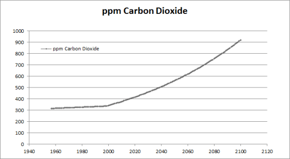
CO2 concentrations increase linearly from 1958 to 2000, and then exponentially until 2100, with a doubling of CO2 (with respect to 1958) around 2062. (This data was output as a spreadsheet, and I got Excel to generate the graph, so it looks nicer than the others.)

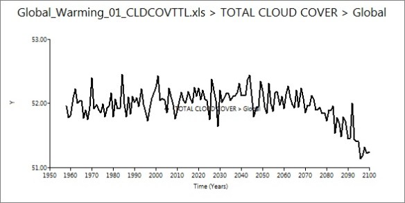
Global cloud cover held steady until around 2070, when it decreased. I can’t figure out why this would be, as the water vapour content of the air should be increasing with warming – wouldn’t there be more clouds forming, not less?

Global precipitation increased, as I expected. This is an instance where I wish the maps would have worked, because it would be neat to look at how precipitation amount varied by location. I’ve been pretty interested in subtropical drought recently.

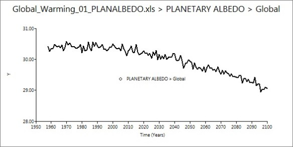
Albedo decreased about 1% – a nice example of the ice-albedo feedback (I presume) in action.

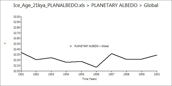
I also ran a simulation of the Last Glacial Maximum, from 21 thousand years ago. This run was much quicker than the first, as (since it was modeling a stable climate) it only simulated a decade, rather than 150 years. It took a few hours, and the same bugs in output were apparent. Time series graphs are less useful when studying stable conditions, but I found the albedo graph interesting:

Up a few percent from modern values, as expected.

It’s fairly expensive to purchase a licence for EdGCM, but they offer a free 30-day trial that I would recommend. I expect that it would run better on a  Mac, as that’s what they do most of the software development and testing on.

Now that I’ve played around with EdGCM, I’m working on porting CESM to a Linux machine. There’s been trial and error at every step, but everything went pretty smoothly until I reached the “build” phase, which requires the user to edit some of the scripts to suit the local machine (step 3 of the user guide). I’m still pretty new to Linux, so I’m having trouble working out the correct program paths, environment variables, modules, and so on. Oh well, the more difficult it is to get working, the more exciting it is when success finally comes!

I am also doing lots of background reading, as my project for the summer will probably be “some sort of written something-or-other” about climate models. Steve has a great collection of books about climate change, and keeps handing me interesting things to read. I’m really enjoying The Warming Papers, edited by David Archer and Ray Pierrehumbert. The book is a collection of landmark papers in climate science, with commentary from the editors. It’s pretty neat to read all the great works – from Fourier to Broecker to Hansen – in one place. Next on my list is A Vast Machine by Paul Edwards, which I’m very excited about.

A quick question, unrelated to my work – why do thunderstorms tend to happen at night? Perhaps it’s just a fluke, but we’ve had a lot of them recently, none of which have been in the daytime. Thoughts?

Quality, Transparency, and Rigour

The Intergovernmental Panel on Climate Change (IPCC) reports are likely the most cited documents on the subject of global warming. The organization, established by the United Nations, doesn’t do any original research – it simply summarizes the massive amount of scientific literature on the topic. Their reports, written and reviewed by volunteer scientists, and published approximately every six years, are a “one-stop shop” for credible information about climate change. When you have a question about climate science, it’s far easier to find the relevant section of the IPCC than it is to wade through thousands of results on Google Scholar.

The main problem with the IPCC, in my opinion, is that their reports are out of date as soon as they’re published, and then everyone has to wait another six years or so for the next version, which is subsequently out of date, and so on. Additionally, because there are so many authors, reviewers, and stakeholders involved in the IPCC, the reports come to reflect the lowest-common-denominator scientific understanding, rather than the median opinion of experts. In particular, government officials oversee the writing and reviewing of the Summary for Policymakers, to make sure that it’s relevant and clear. However, some governments are beginning to abuse their power in this process. The late Stephen Schneider, in his 2009 book Science as a Contact Sport, recounts his experiences with government representatives who absolutely refuse to allow certain conclusions to be published in the IPCC, regardless of their scientific backing.

The result is that the IPCC reports frequently underestimate the severity of climate change. For example, in the most recent report, the worst-case estimate of sea level rise by the end of this century was 0.59 m. Since then, scientists have revised this estimate to 1.9 m, but it won’t show up in the report until the next edition comes out around 2014.

Another example concerns Arctic sea ice: the worst-case scenario from the IPCC was an ice-free Arctic in the summer beginning around 2100. These estimates have come down so rapidly that there’s an outside chance the summer sea ice could be gone before the next IPCC report has a chance to correct it (presentation by Dr. David Barber, media coverage available here). It will more likely disappear around 2035, but that’s still a drastic change from what the IPCC said.

Despite this conservative stance, there are still some who think the IPCC is alarmist (this is usually paired with something about a New World Order and/or socialists using a carbon tax to take over the world). Naturally, the IPCC has become a favourite target of climate change deniers, who wish to obscure the reality of human-caused global warming. Last year, they claimed to have found all kinds of errors in the latest report, somehow proving that global warming wasn’t happening. In fact, most of these so-called “errors” were nothing of the sort, and the worst of the two real mistakes in the report involved a typo regarding which year certain glaicers were expected to disappear. Not bad, for a three-thousand-page document, but it created quite the media firestorm. Apparently scientists are expected to have 100% accuracy at all times, or else they are frauds.

Just a few weeks ago, the IPCC made some changes to their policies in response to these events. Their press release about the new policies featured the phrase “Boost Quality, Transparency and Rigour” in the title.

No, no, no. That’s not what the IPCC needs. These are very admirable goals, but they’re doing just fine as it is. Actions to “further minimize any possibility of errors in future reports” should not be their top priority. Further extending the review process will only further delay the publication of each report (making them even more out of date) and further enhance their lowest-common-denominator position. When you have an error rate on the order of 0.67 errors/1000 pages, should you spend your energy getting that all the way down to zero (a virtually impossible task) or on the real issues that need to be addressed?

I think the IPCC should adopt a continually-updating online version of their report. This would solve their chronic problem of being out of date, as well as help the organization adapt to the increasing role of the Internet in our world. Any future errors the deniers liked to yell about would be fixed immediately. Governments would be forming policies based on the best available evidence from today, not a decade ago. Everything would still be in one place, and version control would allow transparency to remain high.

The IPCC should also make it more clear when their estimates are too conservative. When a single sentence that didn’t even make it into the summary is shown to overestimate the problem, the climate science community ties itself up in knots trying to correct its tattered image. But prominent conclusions that underestimate the problem go unacknowledged for decades. If it were the other way around, can you imagine the field day deniers would have?

Luckily, the changes made to IPCC policy are not all aimed at appeasing the bullies. A long-overdue communications plan is in development: a rapid response team and Senior Communications Manager will develop formal strategies for public education and outreach. Hopefully, this will counteract the false claims and defamation the IPCC has been subject to since its creation.

Another new plan is to create an Executive Committee, composed of the Chair, Vice Chairs, Working Group Co-Chairs, and advisory members. This will “strengthen coordination and management of the IPCC” and allow for actions to be taken between reports, such as communication and responding to possible errors. A more structured administration will probably be helpful, given that the only people in the organization currently getting paid for their work are the office staff (even the Chair doesn’t make a cent). Coordinating overworked scientists who volunteer for a scientific undertaking that demands 100% accuracy can’t be an easy task.

Will the IPCC continue to be the best available source of credible information on climate change? Will its structure of endless review remain feasible in a world dominated by instant news? Should we continue to grant our governments control over the contents of scientific reports concerning an issue that they desperately want to avoid? Should we continue to play to the wants and needs of bullies? Or should we let scientists speak for themselves?